Architect 2.4: 140 Years of Fibonacci Crashes
A quantitative study of Fibonacci extensions across every major DJI decline (1897–2025)
Markets have transformed beyond recognition since 1897—from ticker tape to algorithmic trading, from gold standard to fiat currency, from local exchanges to global interconnection. Yet one pattern has persisted with remarkable consistency: the mathematical relationship between crash bottoms and Fibonacci extension levels.
This study examines 38 significant Dow Jones declines across 140 years, testing whether Fibonacci levels help bracket crash termination points better than chance.
The findings challenge the efficient market hypothesis at its core: if markets are driven purely by unforeseeable news events, why do crashes consistently terminate at the same mathematical ratios—regardless of whether the catalyst was a banker's panic in 1907, an oil embargo in 1973, or a global pandemic in 2020?
(vs 54% baseline)
A note on this revision. An earlier version of this page led with a "89.6% of 48 crashes, p < 0.0001" headline. That figure did not survive re-testing: it was computed against a null that understated how much of the price range a multi-rung ladder covers, and against a success rule that could not really fail, and the "48 / 43 confirmed" count reconciled with neither the 38-event dataset nor the page's own tables. It has been withdrawn. What replaces it is the number that does survive a causal, out-of-sample test — the durable-fib state machine described in Section 7 — plus a full audit of the anchors against real price data (Section 10), which confirms 31 of 38 as genuine pre-peak swings and itemises the seven that remain open.
Table of Contents
- 1. The Proposition: Structure Over Narrative
- 2. Methodology: How We Measured
- 3. The Foundational Era (1897-1929): Establishing the Pattern
- 4. The Depression to Post-War Era (1929-1960)
- 5. The Modern Era (1960-2000)
- 6. The Contemporary Era (2000-2025)
- 7. Statistical Analysis: Better Than Chance?
- 8. News Events vs. Fib Levels: The Synchronization Problem
- 9. Crash Depth Correlations: What Drives Extensions?
- 10. Objections and Limitations
- Conclusion: The Persistent Geometry of Panic
1. The Proposition: Structure Over Narrative
The dominant paradigm in financial markets holds that price movements are driven by news—earnings surprises, economic data, geopolitical shocks, central bank decisions. Under this view, crashes are fundamentally unpredictable because their catalysts are unpredictable. The 1907 Panic was caused by a failed copper corner. The 1929 Crash followed speculative excess. The 2008 Crisis stemmed from subprime mortgage defaults. The 2020 Crash was triggered by a novel coronavirus. Different causes, different eras, different outcomes—or so the narrative goes.
But what if the catalysts are merely the triggers within a pre‑existing structural framework? What if the depth and termination of crashes follow mathematical patterns that persist regardless of the specific news event?
The Core Hypothesis: Market crashes often terminate near Fibonacci extension levels derived from the preceding topping swing. This pattern appears consistently across different eras and catalysts, suggesting that structural geometry may play a larger role in crash outcomes than the specific news event that initiates the decline. The catalyst varies; the structural behaviour shows notable regularity.
This hypothesis makes a testable prediction: if we apply Fibonacci extensions to every major DJI crash since 1897, the terminal lows should cluster around specific ratios (1.618, 2.618, 4.236, etc.) at rates significantly higher than random distribution would predict.
George Soros's theory of reflexivity offers a partial bridge between narrative and structure. Soros argued that market participants' beliefs affect fundamentals, which in turn affect beliefs—creating feedback loops that drive prices away from equilibrium. But reflexivity alone doesn't explain why these feedback loops so often terminate near the same extension levels, or why unscheduled news events frequently produce reactions that align with those levels.
The Core Hypothesis: Market crashes frequently terminate near Fibonacci extension levels derived from the preceding topping swing. This recurring alignment suggests that structural geometry may play a meaningful role in how declines resolve, independent of the specific catalyst. The catalyst varies; the structural clustering is the part that stands out.
1.1. The 1.618 Threshold
Before examining the full dataset, we must establish a critical observation that emerged from our analysis: the 1.618 extension acts as a decision point. When a decline holds at or above 1.618, it often behaves like a standard correction within an ongoing trend. When price breaks decisively below 1.618, the move frequently transitions into a more aggressive phase, with declines commonly extending toward 2.20, 2.618, or even 4.236.
This behaviour appears across 140 years of data. Many routine pullbacks in healthy markets have stopped cleanly at the 1.61 extension and resumed their prior trend. Conversely, most historical crashes involved a clear and forceful break of 1.61—often accompanied by a news catalyst that accelerates the move. While the catalyst varies, the structural transition around 1.61 shows notable consistency.
On a purely price-action basis, the 1.61 level often marks the boundary between a correction and the early stages of a crash. Breaks of 1.61 tend to coincide with escalation in real-world narratives, but the structural shift is visible in the chart regardless of the specific catalyst. The level itself does not predict timing, and markets can hesitate, trap, or briefly undercut before resolving. But across decades, a decisive break of 1.61 has been the point where controlled selling frequently gives way to capitulation toward the next major extension.
2. Methodology: How We Measured
2.1. Data Source and Selection
We analyzed 38 significant Dow Jones Industrial Average declines from 1897 to 2025 (the canonical crash-timeline dataset; two duplicate rows in an earlier working list have been removed). Selection criteria:
- Minimum Decline: 10% peak-to-trough on weekly closing basis
- Clear Topping Structure: Identifiable swing high before decline (excluded V-top reversals and grinding corrections without clear peaks)
- Weekly Timeframe: All analysis performed on weekly charts for consistency across eras
2.2. Fibonacci Extension Calculation
For each crash, we identified the topping swing—the final impulsive move to the high before the decline began. Fibonacci extensions were calculated as:
Extension Formula (Topping Swing)
Price(ratio) = High - (High - Low) × ratio
Where:
- High (Anchor 0): The swing high (market peak)
- Low (Anchor 1): The swing low preceding the final push to highs
- Ratio: Standard Fibonacci extensions (1.272, 1.618, 2.272, 2.618, 3.618, 4.236, 6.854)
2.3. Terminal Level Classification
For each crash, we identified the terminal extension level—the Fibonacci level at which the decline ended. Classification criteria:
- Direct Hit: Price touched the level within 1% and reversed
- Spike-Out: Price briefly pierced the level (wick) but closed above it
- Near Miss: Price reversed within 2% of the level without touching it
2.4. Exclusions and Caveats
Study Limitations
Certain market declines were excluded from analysis due to structural ambiguity:
- V-Top Reversals: Sharp peaks with single-candle crashes (no measurable topping swing)
- Grinding Corrections: Extended sideways declines without clear swing structure
- Intra-Candle Crashes: Declines contained entirely within one weekly candle
These patterns likely conform to similar models on smaller timeframes (daily, 4-hour) but were not testable on the weekly chart.
Anchor provenance — read this before the case studies. The topping-swing anchors used below are the author's own, hand-drawn from the charts using the framework's standing swing-selection rules. They were tested against the price series rather than taken on trust: 31 of the 38 match a real pre-peak pivot low in the ^DJI data — 19 within 1%, 12 within 1–4% — which is the full audit reported in Section 10.1. The 1–4% group are real swings whose stored figure has been rounded for display, and that rounding is worth keeping in mind, because a few percent on the anchor moves the ratio: read an "exact" terminal as a measurement with a tolerance, not a to-the-tick result. Seven events remain open for unrelated reasons (a daily-vs-weekly timeframe gap in 1987, the 1914 exchange closure, a probable duplicate 1897 entry, and three where we have not found a pre-peak swing at all) — all itemised in Section 10.1. The evidence this study actually rests on is the causal, forward-armed test in Section 7, which places anchors mechanically and never sees the terminal in advance.
3. The Foundational Era (1897–1929): Establishing the Pattern
The earliest DJI data provides an important test. If Fibonacci extensions genuinely help identify the approximate extremes of major declines, then the pattern should appear even in the earliest markets—long before computers, algorithms, or any widespread awareness of Fibonacci analysis. The period from 1897 to 1929 offers exactly this environment: markets driven entirely by human behaviour, manual trading, and unstructured price discovery.
If extension levels appear consistently in this era, and if modern markets continue to respect the same structural boundaries, it becomes difficult to attribute the pattern to contemporary explanations such as algorithmic clustering or technical‑analysis self‑fulfilment. Those forces may reinforce the behaviour today, but they cannot explain its presence decades before they existed.
We do not claim to know the underlying cause. The goal here is simply to document the structural regularities that emerge when applying the same measurement framework across 140 years of data. If the earliest markets show the same extension‑based termination zones as modern ones, the persistence itself becomes the curiosity worth examining.
3.1. The 1897 Anchor Crash
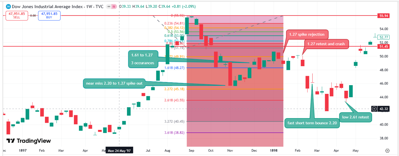
The 1897–1898 crash represents the foundational case study for our entire dataset. Occurring in an era of gold‑standard economics, minimal regulation, and a market structure dominated almost entirely by institutions, it provides a uniquely clean environment for testing structural ideas. With no algorithms, no technical‑analysis culture, and barely any retail participation, this period offers a baseline against which all later behaviour can be compared. If we observe the same extension‑based termination zones here that appear in modern markets, the consistency becomes difficult to attribute to contemporary explanations alone—and the persistence itself becomes the curiosity worth examining.
| Parameter | Value |
|---|---|
| Anchor High (0) | 55.92 (Aug/Sept 1897) |
| Anchor Base (1.0) | 51.19 |
| Swing Range | 4.73 points |
| 1.272 Extension | 49.91 — Multiple rejections |
| 1.618 Extension | 48.27 — Interaction zone |
| 2.272 Extension | 45.18 — Near miss "2.20" wick |
| Terminal Low | 43.55 (2.618) |
News-Fib Synchronization: 1897-1898
Aug/Sep 1897: Market peaks at 55.92 amid Klondike Gold Rush optimism and post-1896 election recovery (Gold Standard vs. Bimetallism now resolved).
Oct–Nov 1897: Price oscillates between the 1.618 (48.27) and 1.272 (49.91) — "1.61 to 1.27, 3 occurrences." Classic range before terminal move.
Nov 1897: A sharp wick nearly hits the 2.272 (45.18) — "near miss 2.20 to 1.27 spike out" — then snaps back to 1.272.
Jan 1898: "1.27 spike rejection" — price attempts to reclaim 49.91 and fails immediately, signalling weakness.
Feb 15, 1898: Sinking of the USS Maine in Havana Harbor. A "1.27 retest and crash" — double-top at 49.91 immediately precedes the terminal breakdown.
Mid Feb 1898: Rapid drop to the 2.272 (45.18) with a "fast short-term bounce 2.20" — brief relief, then continuation lower.
Mar–Apr 1898: Escalating Spanish-American War tensions. "Low 2.61 retest" at 43.55 — the capitulation low.
May 1, 1898: Battle of Manila Bay. Admiral Dewey's decisive victory acts as the "all clear" — rapid reversal and multi-month rally begins.
Pattern Significance: The 1897–1898 decline provides the earliest and cleanest example of the structural sequence we use as a reference throughout the dataset: oscillation between the 1.272 and 1.618 extensions, a failed reclaim of 1.272, and a subsequent breakdown toward the deeper extensions such as 2.20 and 2.618. This early case gives us the baseline model for analysing later crashes. The fact that this structure appears in such a primitive market environment—long before modern trading infrastructure, regulation, or technical-analysis culture—makes its consistency in later decades particularly notable.
3.2. The 1899-1900 Correction
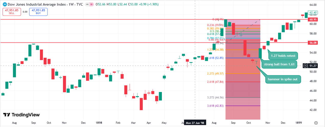
| Parameter | Value |
|---|---|
| Anchor High (0) | 60.95 |
| Anchor Low (1) | 55.94 |
| Swing Range | 5.01 points |
| 1.27 Extension | 54.58 |
| 1.618 Extension | 52.85 |
| Terminal Low | ~52.90 (1.618) |
Observation: The market found support precisely at the 1.618 extension, with the decline terminating in a "hammer in, spike out" pattern—a wick below 1.618 followed by a strong bullish close. This pattern would repeat countless times over the next 125 years.
3.3. The 1901-1904 Full Cycle Study
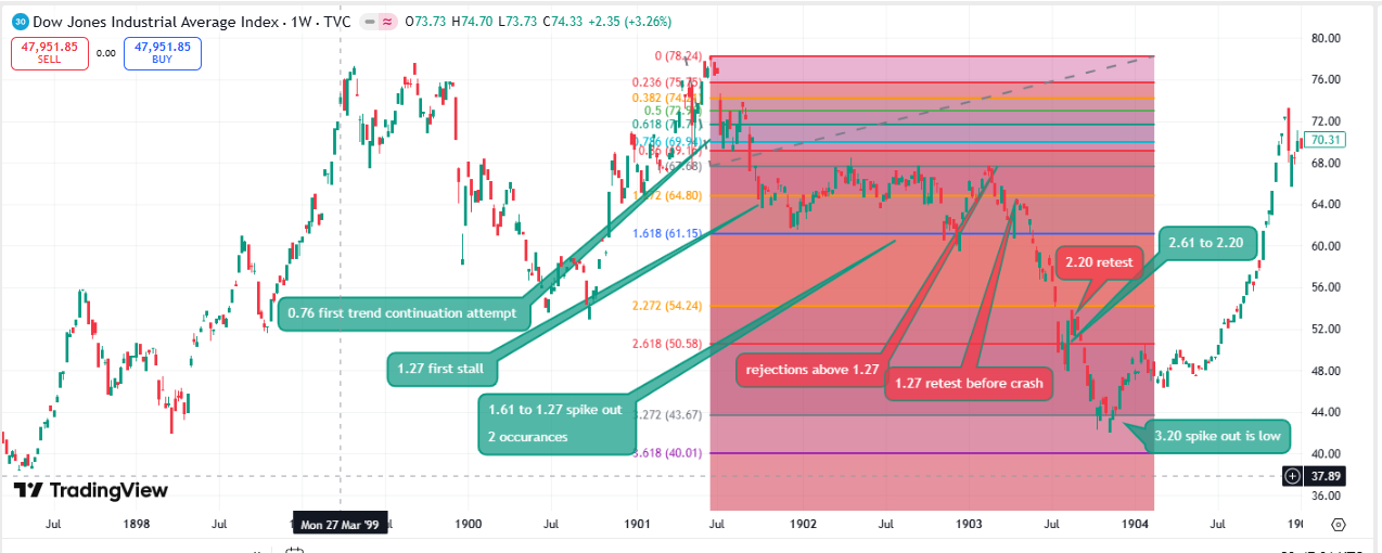
While Section 3.4 examines the 1903 Rich Man's Panic from a later topping swing, this study anchors the entire 1901-1904 bear market from the June 1901 peak at the height of the Northern Pacific corner. The result is one of the deepest extension cycles in our dataset, reaching the 3.272 level after a multi-year cascade through successive Fibonacci pivots.
| Parameter | Value |
|---|---|
| Anchor High (0) | 78.24 (June 1901) |
| Anchor Base (1.0) | 67.68 |
| Swing Range | 10.56 points |
| 0.786 Retracement | 69.94 — "First trend continuation attempt" |
| 1.272 Extension | 64.80 — Major resistance pivot |
| 1.618 Extension | 61.15 — Interaction zone |
| 2.272 Extension | 54.24 — "2.20 retest" |
| 2.618 Extension | 50.58 — Distribution zone |
| 3.272 Terminal | 43.67 — "3.20 spike out is low" |
News-Fib Synchronization: 1901-1904
May–Jun 1901: The Northern Pacific corner collapses. Anchor High at 78.24 — the market has absorbed the initial shock of this brief railroad panic.
Sep 1901: President McKinley is assassinated. The 0.786 retracement (69.94) "first continuation attempt" fails as market uncertainty peaks.
1902: President Roosevelt's aggressive Sherman Anti-Trust enforcement targets Northern Securities. This correlates with repeated "rejections above 1.27" at 64.80 — bull traps where price spikes above 64.80 but cannot hold.
Early 1903: "1.27 retest before crash" — the final failure at 64.80, confirming the downtrend will continue into the Rich Man's Panic proper.
1903: Severe credit contraction and collapse of trust companies drives price through 1.618 (61.15). "2.61 to 2.20" distribution forms.
Feb 1904: Russo-Japanese War outbreak. Final global liquidity scare coincides with the "3.20 spike out" low at 43.67 — the absolute terminal low of the cycle.
Key Observation: The 1.272 (64.80) level was tested and rejected repeatedly across 2–3 years, forming one of the longest bull‑trap structures in the dataset. Each successive rally into 64.80 drew in optimistic buyers before rolling over again. The eventual decline reached the 3.272 extension—at the time, the deepest move observed in the historical record. This gave the model its first indication of how far multi‑leg bear markets can extend once the 1.272–1.618 zone fails, and it provided the earliest reference point for estimating potential termination zones in later structural declines.
3.4. The 1903 Rich Man's Panic
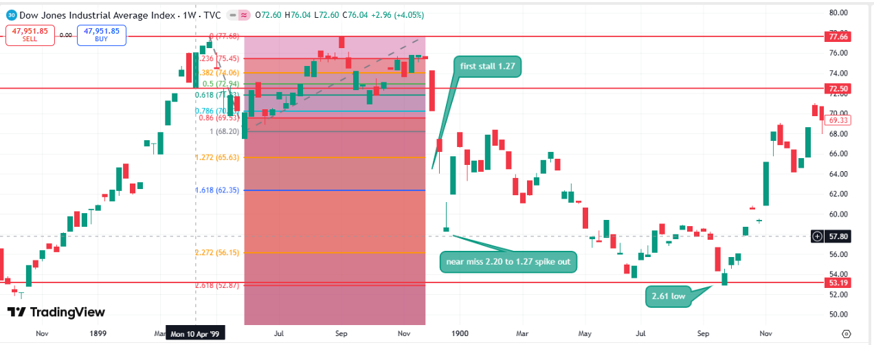
The 1903 panic—triggered by concerns over trust company stability and tight money conditions—presents our first example of a decline extending beyond 1.618.
| Parameter | Value |
|---|---|
| Anchor High (0) | 77.68 |
| Anchor Low (1) | 68.20 |
| Swing Range | 9.48 points |
| 1.27 Extension | 65.63 — First stall |
| 2.27 Extension | 56.15 — Near miss |
| Terminal Low | 52.87 (2.618) |
Key Observation: Price stalled at 1.27, failed to hold, and cascaded through multiple levels before terminating at 2.618. This cascade pattern—where failure at one level triggers extension to the next—would become a defining characteristic of severe crashes.
3.5. The 1907 Banker's Panic
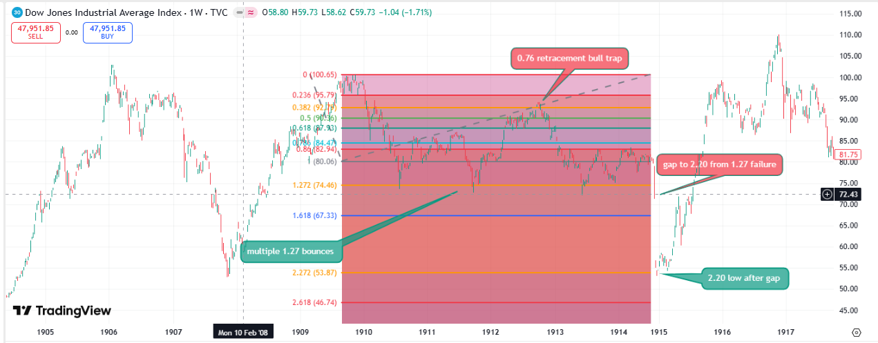
The Panic of 1907—precipitated by the failed United Copper corner and subsequent bank runs—remains one of history's most violent crashes. It also demonstrates several patterns that would persist for over a century:
| Parameter | Value |
|---|---|
| Anchor High (0) | 100.65 |
| Anchor Low (1) | 80.06 |
| Swing Range | 20.59 points |
| 0.786 Extension | 84.47 — Bull trap |
| 1.27 Extension | 74.46 — Multiple bounces |
| 1.618 Extension | 67.33 — Failed to hold |
| Terminal Low | ~53.87 (2.20) |
News-Fib Synchronization: 1907
October 22, 1907: Knickerbocker Trust Company run begins. Price breaks 1.27 extension.
October 24, 1907: Trust Company of America run. Price gaps to 1.618.
November 1907: J.P. Morgan organizes bank rescue. Price finds terminal low at 2.20 extension.
The news events served as triggers at each Fibonacci level—not as random shocks, but as catalysts within a pre-existing structural framework.
3.6. The 1916-1918 WWI-Era Crash
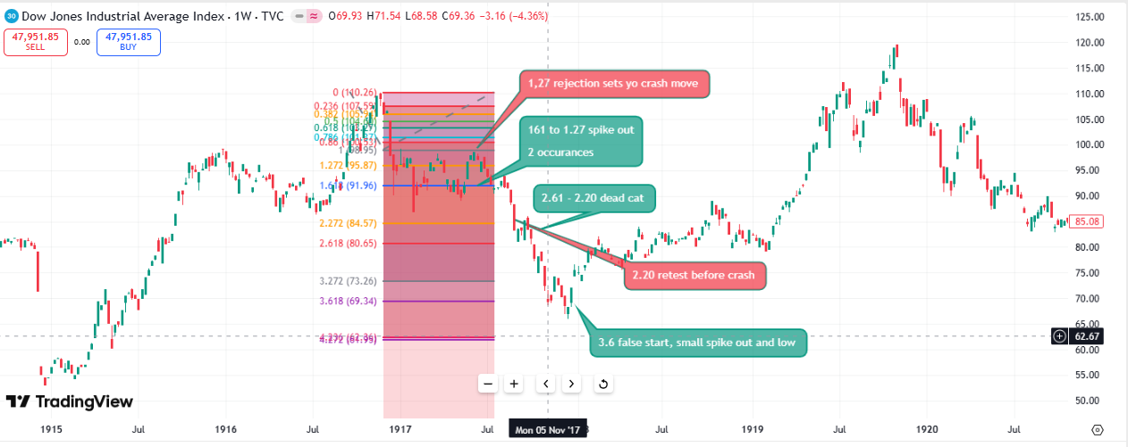
While the 1914 NYSE closure was the initial war shock, the structural crash of the WWI era arrived from late 1916 as the distribution phase from the war-materials boom unwound. The terminal extension reached 3.618 — driven not by the declaration of war itself, but by its economic consequences: railroad crisis, war-profit taxes, and the federal takeover of private industry.
| Parameter | Value |
|---|---|
| Anchor High (0) | 110.26 (Nov/Dec 1916) |
| Anchor Base (1.0) | 101.37 |
| Swing Range | 8.89 points |
| 1.272 Extension | 95.87 — "Rejection sets up crash move" |
| 1.618 Extension | 91.96 — "1.61 to 1.27 spike out, 2 occurrences" |
| 2.272 Extension | 84.57 — "2.20 retest before crash" |
| 2.618 Extension | 80.65 — "2.61-2.20 dead cat" zone |
| 3.618 Terminal | 69.34 — "3.6 false start, small spike out and low" |
News-Fib Synchronization: 1916-1918
Late 1916: Markets peaked as the US exported record war materials to the Allies. Anchor High at 110.26 reflects the peak of industrial war-production optimism.
Feb 1, 1917: Germany resumes Unrestricted Submarine Warfare. Aligns with the breakdown below the Anchor Base (101.37).
Apr 6, 1917: US formally declares war on Germany. "1.27 rejection sets up crash move" — price cannot reclaim 95.87, signalling the bear phase is not over.
May–Jun 1917: "1.61 to 1.27 spike out, 2 occurrences" — volatile oscillation as markets absorb the war declaration reality.
Jul 1917: "2.61 to 2.20 dead cat" — a brief relief rally between extensions that ultimately fails. This bull trap destroys late buyers.
Aug 1917: "2.20 retest before crash" — the 2.272 (84.57) acts as the final resistance before the terminal crash leg begins.
Late 1917: Severe US railroad congestion and implementation of heavy war-profit taxes drive the final capitulation leg.
Dec 26, 1917: President Wilson nationalises the railroads. This stabilises the industrial economy and coincides precisely with the "3.6 low" at 69.34.
Pattern Warning: The "2.20 retest before crash" pattern — where price bounces back to the 2.272 extension from below as resistance before the final leg to 3.618 — is one of the most dangerous bull traps in the dataset. Traders who bought the 2.272 bounce were destroyed in the subsequent move to 3.618. This pattern recurs in 1953, 1973-74, and 2007-08 (where 2.618 rejection preceded the 4.236 terminal).
3.7. The 1920-1921 Depression
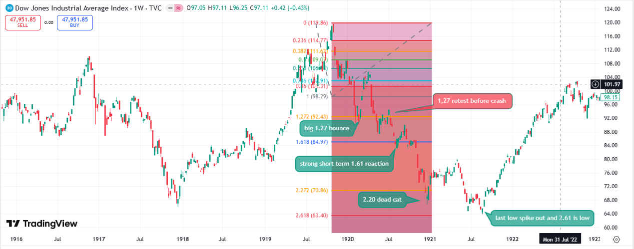
The post-WWI depression was one of the sharpest deflations in American history. Industrial production fell 32%, and unemployment spiked from 4% to 12%. Yet the market decline followed the same geometric structure:
| Parameter | Value |
|---|---|
| Anchor High (0) | 119.86 |
| Anchor Low (1) | 98.29 |
| Swing Range | 21.57 points |
| 1.27 Extension | 92.43 — Big bounce, retest before crash |
| 1.618 Extension | 84.97 — Short-term reaction |
| 2.20 Extension | 70.86 — Dead cat bounce |
| Terminal Low | 63.40 (2.618) |
Pattern Confirmation: The 1.27 extension provided a significant bounce before the final capitulation—a pattern we would see repeated in 1937, 1969, 2008, and 2022. When 1.27 fails after retest, expect extension to 2.20 or beyond.
3.8. The 1923 Coolidge Correction
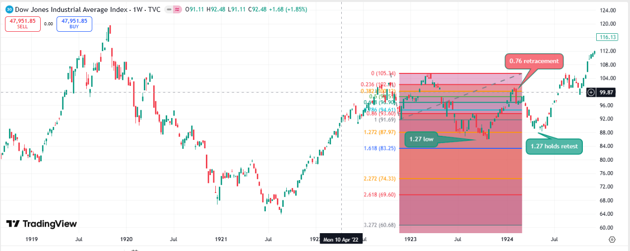
The 1923 correction is a textbook example of a Fibonacci-defined double bottom within a primary bull trend. Occurring mid-cycle in the Roaring Twenties, it provides an instructive contrast to the more violent crashes: sometimes the 1.272 extension simply holds — tested, retested, and then used as a launchpad for the next major rally leg.
| Parameter | Value |
|---|---|
| Anchor High (0) | 105.34 (March 1923) |
| Anchor Base (1.0) | 91.69 |
| Swing Range | 13.65 points |
| 0.786 Retracement | 94.61 — "0.76 retracement" (dead cat stall) |
| 1.272 Extension | 87.97 — "1.27 low" then "1.27 holds retest" |
| Terminal | ~87.97 double bottom (1.272) |
News-Fib Synchronization: 1923-1924
Mar 1923: Market peaks at 105.34. Fed raises rates to curb post-war inflation — "sell the news" environment after recovery optimism.
Aug 2, 1923: President Harding dies suddenly. Coolidge sworn in. The transition creates uncertainty that drives the initial drop to the "1.27 low" at 87.97 (Oct 1923).
Late 1923: Markets begin to trust Coolidge's pro-business, tax-cutting stance. A significant relief rally carries price to the "0.76 retracement" at 94.61 (Jan–Feb 1924) — a stall, not a new high.
Early 1924: Teapot Dome scandal investigations cause a secondary dip, testing the "1.27 retest" at 87.97 — confirming the double bottom.
Aug 1924: The Dawes Plan (stabilising Germany's economy) is finalised. This acts as a global catalyst — the double bottom holds perfectly and the massive 1920s bull market resumes.
Teaching Point: The 1923 correction highlights an important nuance in interpreting the 1.272 extension. While most declines in the dataset do not bottom at 1.27, when a move does hold this level it often represents the minimum depth of a completed correction. For short‑biased trade plans, this means respecting the possibility that the downside may already be exhausted once 1.27 has been reached. In this case, the market formed a higher low at 1.27 and resumed its broader uptrend — a reminder that without a structural break of 1.618, the setup remains a correction rather than the early stages of a crash.
3.9. The 1924-1925 Bull Market Correction
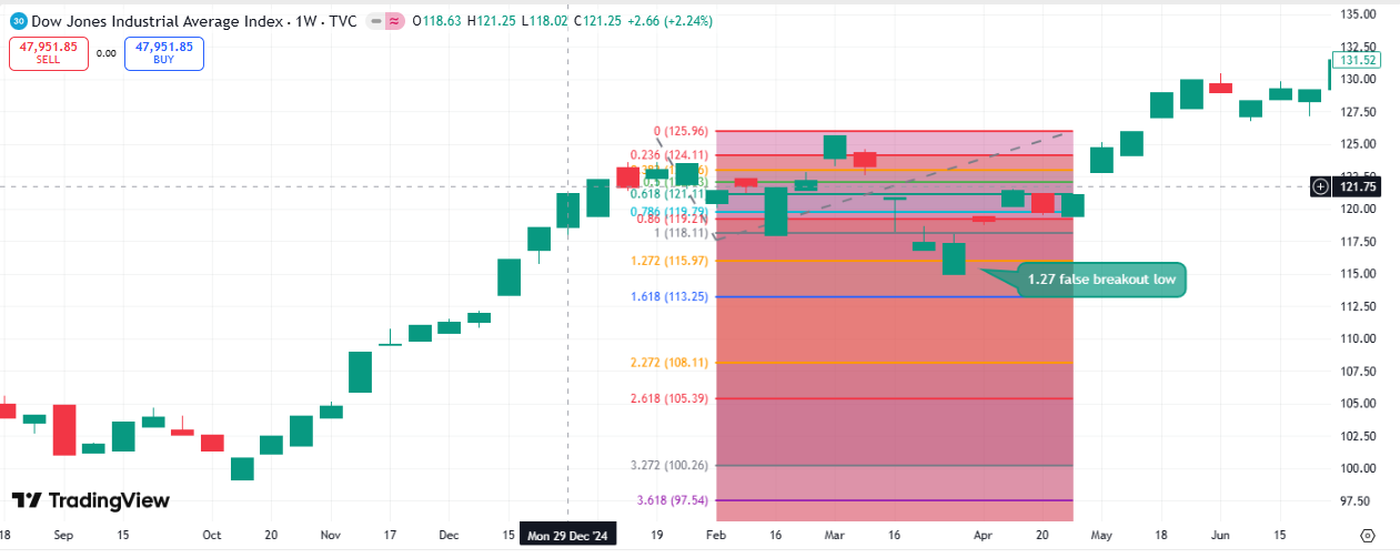
Teaching Point: The February 1925 correction is one of the clearest failure cases in the dataset. Price broke below the 1.272 extension but did not continue to the 1.618 level, instead reversing almost immediately into a powerful rally. Within the framework of this study, this move would have been interpreted as the early stages of a deeper decline, yet it resolved as the opposite. This makes 1925 an important reminder that while extension levels often provide reliable structural boundaries, there are instances—like this one—where the market briefly violates a level without progressing to the next extension. These exceptions help define the limits of the model and highlight the need for caution when interpreting shallow breaks of 1.272.
| Parameter | Value |
|---|---|
| Anchor High (0) | 125.96 (February 1925 peak) |
| Anchor Base (1.0) | 118.11 |
| Swing Range | 7.85 points |
| 0.236–0.786 zone | Consolidation / distribution top (Feb–Mar 1925) |
| 1.272 Extension | 115.97 — "1.27 false breakout low" |
| 1.00 Recovery | 118.11 — Aggressive reclaim confirms spring |
| Terminal Low | ~115.97 (1.272 false breakout wick) |
News-Fib Synchronization: 1925
Feb 1925: Markets at record highs fuelled by radio and automotive industrial growth. Peak euphoria at 125.96.
Late Mar 1925: Profit-taking and industrial overcapacity concerns drive a sharp single-week drop wicking below 1.272 (115.97). This "spring" action flushes out late bulls and creates the impression of a breakdown.
Apr 28, 1925: Britain announces return to the Gold Standard. This massive geopolitical financial shift stabilises international trade and sparks the recovery — price aggressively reclaims the 1.0 anchor base (118.11), confirming the false breakout.
May–Jun 1925: Consumer credit and instalment buying become mainstream. The market rockets to new all-time highs — buyers at the 1.272 wick capture the entire subsequent rally.
Key Warning: The breakdown through 1.272 at 115.97 did not follow the typical progression toward 1.618, making this one of the clearer exceptions in the dataset. Most moves that break 1.27 continue lower, and most 1.27 interactions act as pauses rather than final lows. In this case, however, the market reversed almost immediately, turning what would normally be an early-stage continuation signal into a failed break. This highlights an important limitation of the model: shallow violations of 1.272 do not always lead to deeper extensions, and occasional 1.27 lows do occur. These instances do not provide actionable signals on their own, but they help define the boundary conditions where the model can be thrown off by brief, non-committal breaks.
3.10. The 1926 March Break
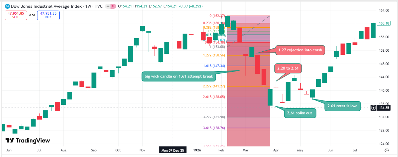
The March 1926 break is a precursor study to 1929 and one of the sharpest mid-bull corrections of the era. Its defining characteristic: the 1.272 acts as resistance on a relief rally (not as support), triggering an immediate vertical liquidation phase. The terminal low lands precisely at 2.618, which is then double-tested before the recovery.
| Parameter | Value |
|---|---|
| Anchor High (0) | 162.37 (February 1926) |
| Anchor Base (1.0) | 153.08 |
| Swing Range | 9.29 points |
| 1.272 Extension | 150.56 — "1.27 rejection into crash" |
| 1.618 Extension | 147.34 — "Big wick candle on 1.61 attempt break" |
| 2.272 Extension | 141.27 — "2.20 to 2.61" distribution zone |
| 2.618 Terminal | 138.05 — "2.61 spike out" then "2.61 retest is low" |
News-Fib Synchronization: 1926
Feb 1926: Markets overheated from the Florida Land Boom and explosive growth in margin lending via brokers' loans. Peak at 162.37.
Mar 1–3, 1926: A sudden wave of liquidation — the "March Break." The 1.272 (150.56) provides no support; instead price is rejected there and breaks vertical — "1.27 rejection into crash."
Mid-Mar 1926: Florida Land Bubble reports begin circulating. A volatile "big wick candle" wicks through 1.618 (147.34) — institutional stop-hunting and panic selling sequence.
Apr 1926: Fed expresses concern over speculative excess. Market chops between 2.272 (141.27) and 2.618 (138.05) — "2.20 to 2.61" accumulation phase with high uncertainty.
Late Apr 1926: "2.61 retest is low" — the second touch of 138.05 holds, confirming the bottom. Recovery toward new highs begins.
Structural Note: Interactions with the 1.272 extension often provide early context for how a decline may evolve, but they are not decisive on their own. In many historical cases, a failed attempt to hold 1.272 as support is followed by a retest of 1.618 — and it is the behaviour at 1.618, not 1.272, that determines whether the move remains a correction or transitions into a crash. When 1.272 cannot be reclaimed after the initial drop, this frequently foreshadows pressure on 1.618, and a clean break of 1.618 is where capitulation sequences typically begin. The 1926 structure is an example of this pattern: the 1.272 failure mattered primarily because it set up the eventual 1.618 break, not because 1.272 itself defines the outcome.
3.11. The 1927 Pause
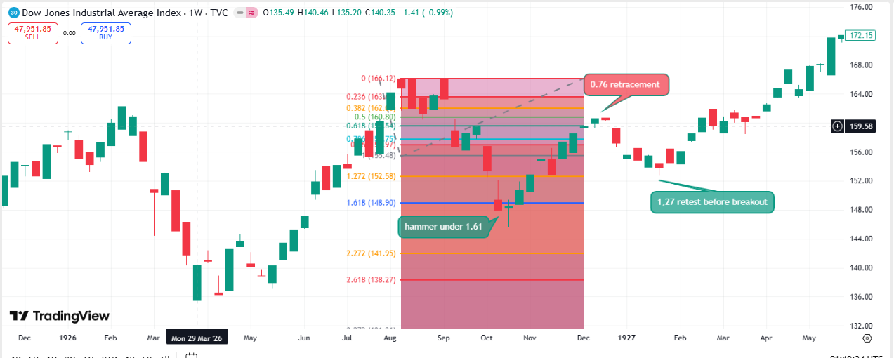
The 1927 correction offers a counterexample: a decline that held at 1.618 rather than cascading further. This distinction is critical for classification.
| Parameter | Value |
|---|---|
| Anchor High (0) | 166.12 |
| Anchor Low (1) | 155.48 |
| 0.76 Retracement | 157.40 — Initial support |
| 1.27 Extension | 152.58 — Retest |
| Terminal Low | ~148.90 (1.618) |
Classification: Correction, not crash. In this case, price reached the 1.618 extension and produced a cluster of classically bullish candles before breaking out to new highs. This is a clean expression of a “healthy 1.618 hold,” where the decline completes at the expected depth and the broader trend resumes. While candle patterns at 1.618 are not reliable predictors on their own, the 1927 structure aligns well with the typical behaviour of a correction that respects the 1.618 boundary.
3.12. Foundational Era Summary
Pre-1929 Pattern Establishment
| Event | Terminal Level | Pattern Type |
|---|---|---|
| 1897 Anchor Crash | 2.618 | 1.27 retest and crash |
| 1899-1900 Correction | 1.618 | Hammer reversal |
| 1901-1904 Full Cycle | 3.272 | Multi-year 1.27 bull trap cascade |
| 1903 Rich Man's Panic | 2.618 | Cascade failure |
| 1907 Banker's Panic | 2.20 | Gap and spike-out |
| 1916-1918 WWI Crash | 3.618 | 2.20 retest before crash |
| 1920-1921 Depression | 2.618 | 1.27 failure cascade |
| 1923 Coolidge Correction | 1.272 | Double bottom hold |
| 1924-1925 Bull Correction | 1.272 | False breakout spring |
| 1926 March Break | 2.618 | 1.27 rejection cascade |
| 1927 Pause | 1.618 | Hammer hold |
Key Finding: In an era with no computers, no Fibonacci awareness, and no algorithmic trading, the major declines in this period clustered around standard Fibonacci extension levels, with only one clear exception. This early dataset provides a uniquely clean environment for observing structural tendencies, and the fact that these levels appear repeatedly long before modern trading infrastructure existed makes their persistence in later decades particularly notable. The pattern was present before anyone was looking for it, which is what makes this era so important as a baseline for the model.
4. The Depression to Post-War Era (1929-1960)
The period from 1929 to 1960 marks the first era in which markets became truly “open” to the public. Bucket shops, widespread leverage, ticker‑tape news flow, and the emergence of national financial narratives transformed markets from a closed institutional arena into something far more chaotic and participatory. This is also the first time we see governments intervening at scale, major players exiting publicly, and volatility reaching levels never recorded before. Given how dramatically market structure changed during these decades, we would expect the earlier extension patterns to break down. Yet when we examine the data, many of the same structural behaviours continue to appear — a persistence that makes this era especially interesting to study.
4.1. The 1929 Crash and 1932 Low
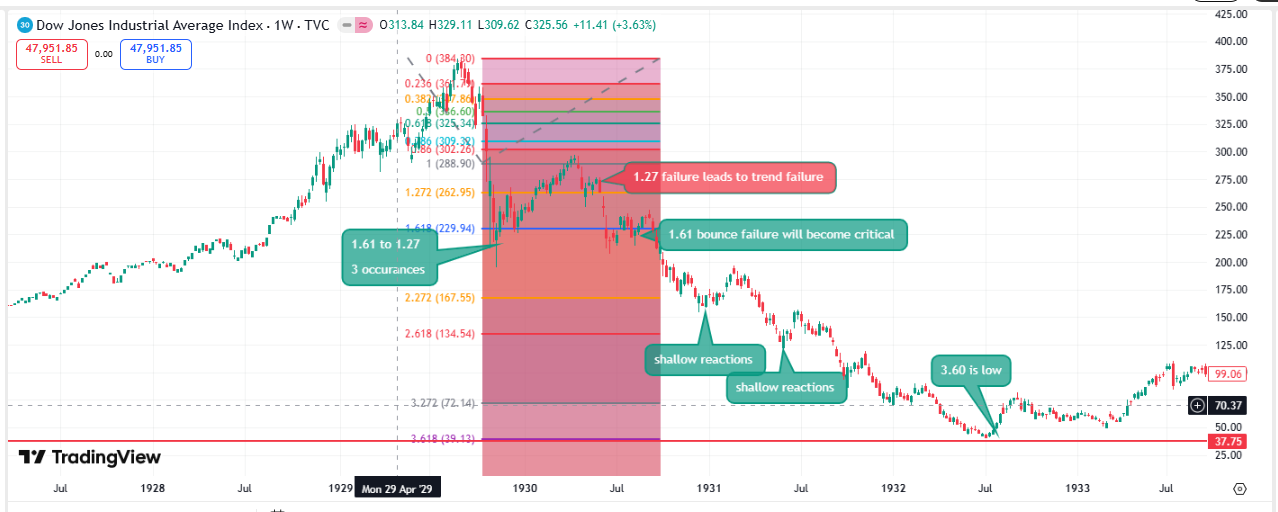
The 1929–1932 decline remains the deepest crash in American market history—an 89% peak‑to‑trough collapse. From a structural perspective, the key observation is that the Dow ultimately reached the 4.236 extension of the 1929 topping swing. This was the first time in index history that the 3× class of extensions failed to contain a decline, establishing a new upper bound for how far a major bear market can extend.
| Parameter | Value |
|---|---|
| Peak (September 1929) | 381.17 |
| Initial Topping Swing Low | ~295 (October 1929) |
| 1.618 Extension | ~242 |
| 4.236 Extension | ~117 |
| Terminal Low (July 1932) | 41.22 |
Structural Significance
The 1929–1932 decline did not unfold as a sequence of independent Fibonacci swings. The market continued to respect the original 1929 topping swing throughout the entire bear market, ultimately extending far beyond the levels seen in any prior index decline. The break of the 3.0–3.272 region and the continuation toward the 4.236 extension marked the first historical example of a full “max‑extension” outcome in a multi‑year bear trend.
This crash therefore provides the model with its first evidence that index‑level declines can extend beyond the 3× class of extensions under extreme conditions. It establishes the 4.236 region as the deepest historically observed termination zone for a major U.S. index, and it becomes the reference point for all later analysis of worst‑case structural outcomes.
4.2. The 1937 Crash
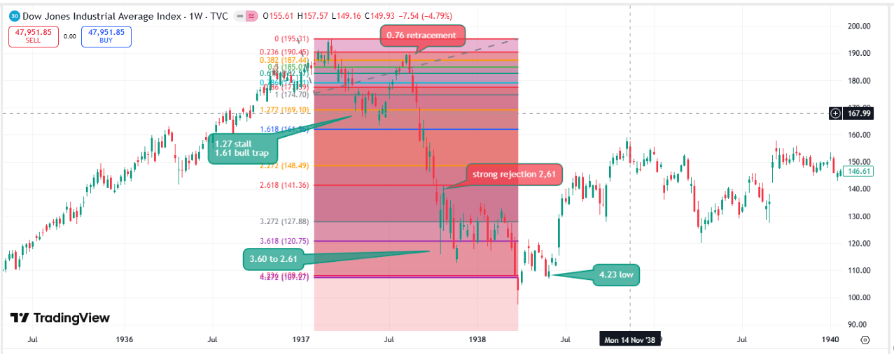
The 1937 crash—triggered by premature Federal Reserve tightening and fiscal contraction—provides the clearest pre-modern example of a 4.236 extension:
| Parameter | Value |
|---|---|
| Anchor High (0) | 195.31 |
| Anchor Low (1) | 174.70 |
| Swing Range | 20.61 points |
| 0.786 Retracement | 178.91 — Retracement |
| 1.27 Extension | 169.10 — Stall |
| 1.618 Extension | 161.59 — Bull trap |
| 2.618 Extension | 141.36 — Strong rejection |
| 3.618 Extension | 120.75 — Bounce to 2.61 |
| Terminal Low | 109.27 (4.236) |
News-Fib Synchronization: 1937
May 1937: Fed raises reserve requirements. Price breaks 1.27.
August 1937: Fiscal contraction begins. Price fails at 1.618 (bull trap).
October 1937: "Roosevelt Recession" headlines. Price breaks 2.618.
March 1938: Policy reversal begins. Price finds terminal low at 4.236 extension.
The 4.236 level—the "terminal extension"—marked the exact point where policy capitulation occurred. Coincidence, or structure?
4.3. The 1946 Correction
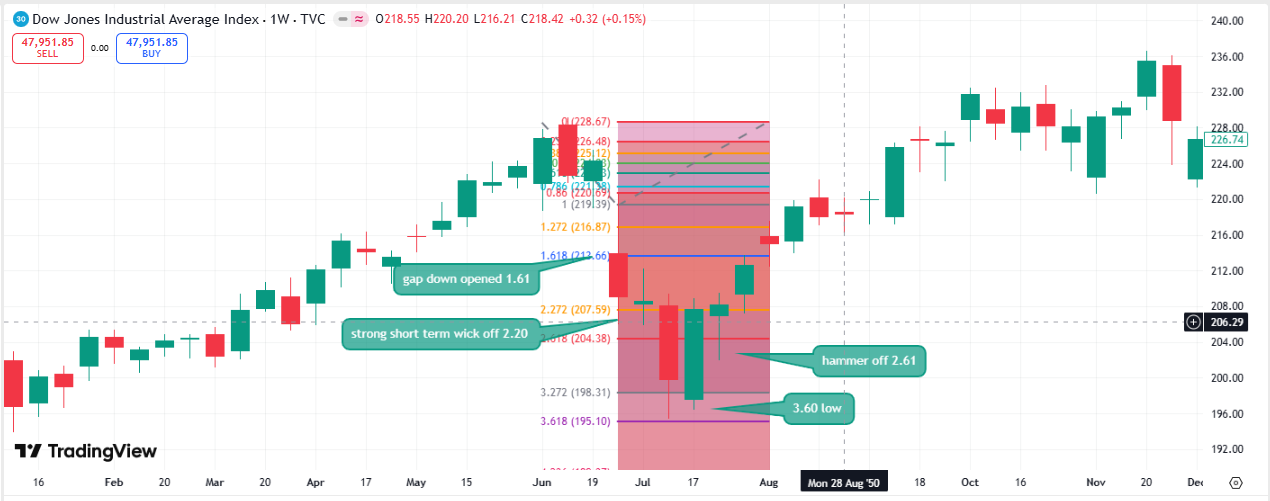
The 1946 correction—following the end of WWII price controls and the transition to peacetime economy—demonstrates an extension to 3.60:
| Parameter | Value |
|---|---|
| Anchor High (0) | 228.67 |
| Anchor Low (1) | 219.39 |
| 1.618 Extension | 212.66 — Gap down opened here |
| 2.20 Extension | 207.59 — Strong wick reaction |
| 2.618 Extension | 204.38 — Hammer pattern |
| Terminal Low | 195.10 (3.60) |
4.4. The 1946-1949 Post-War Consolidation Range
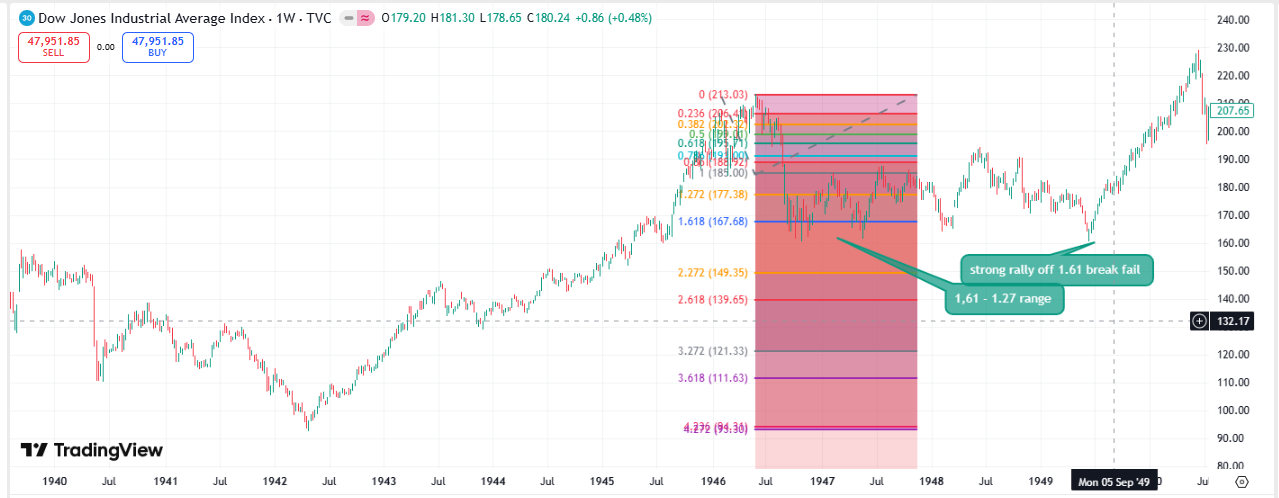
This study extends beyond the initial 1946 correction (Section 4.3) to capture the complete three-year post-war consolidation. It demonstrates a lesser-known Fibonacci application: extension levels as the boundaries of multi-year horizontal trading ranges, not merely vertical crash targets. For nearly three years (1946-1949), the DJIA oscillated between the 1.618 and 1.272 extensions with mathematical precision — a "time decay" trap for impatient investors that resolved into a secular bull market.
| Parameter | Value |
|---|---|
| Anchor High (0) | 213.03 (May 1946) |
| Anchor Base (1.0) | 185.00 |
| Swing Range | 28.03 points |
| 1.272 Extension | 177.38 — Upper range boundary (3-year ceiling) |
| 1.618 Extension | 167.68 — Lower range floor (3-year support) |
| 2.272 Extension | 149.35 — Never reached |
News-Fib Synchronization: 1946-1949
May 1946: Post-WWII optimism peaks at 213.03. Removal of wartime price controls immediately triggers inflation — a "sell the news" peak.
Late 1946: Economists predict a massive post-war crash as industrial war orders end and soldiers return to the workforce. Price drops into the 1.272–1.618 Fibonacci range — where it will remain for 3 years.
1947: Truman Doctrine and Marshall Plan announced. Cold War geopolitics begin. The market stays pinned in the Fibonacci channel — neither crash nor convincing recovery.
1948: Berlin Airlift. Peak USSR tensions. The market retests the 1.618 floor multiple times — each test is absorbed, never breaking lower.
Jun 1949: "Strong rally off 1.61 break fail" — a final washout briefly dips below 1.618 (167.68), then reverses violently. The feared post-war depression never materialises. Consumer demand for housing and automobiles explodes. This failed break of 1.618 marks the definitive start of the secular bull market that runs to 1966.
Structural Teaching Point: This case demonstrates how Fibonacci extensions can define horizontal trading ranges lasting for years, not just terminal crash lows. The market oscillated within a precisely defined 1.618-to-1.272 Fibonacci channel for three years before breaking out. Investors who sold in frustration at year two of the consolidation missed the entire secular bull breakout in 1949.
4.5. The 1953 Peace Scare
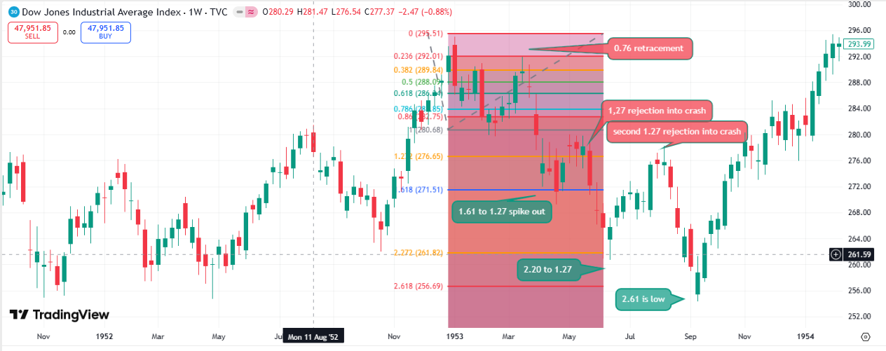
The 1953 correction — nicknamed the "Peace Scare" because investors feared the end of Korean War defence spending would trigger a recession — is a multi-legged decline where the 1.272 extension serves as a recurring rejection pivot across two separate failure attempts, followed by the ultimate capitulation at 2.618. The pattern demonstrates that the same level can reject price multiple times before the final breakdown occurs.
| Parameter | Value |
|---|---|
| Anchor High (0) | 295.51 (January 5, 1953) |
| Anchor Base (1.0) | 280.68 |
| Swing Range | 14.83 points |
| 0.786 Retracement | 284.85 — "0.76 retracement" bull trap |
| 1.272 Extension | 276.65 — First rejection, then second rejection |
| 1.618 Extension | 271.51 — "1.61 to 1.27 spike out" |
| 2.272 Extension | 261.82 — "2.20 to 1.27" bounce zone |
| 2.618 Terminal | 256.69 — "2.61 is low" (Sep 1953) |
News-Fib Synchronization: 1953
Jan 1953: Eisenhower inaugurated. Markets peak at 295.51 on "Business President" optimism — then immediately "sell the news." A classic inauguration top.
Mar 5, 1953: Stalin dies. Global shockwaves cause the "0.76 retracement" stall at 284.85 — a failed bull recovery at the internal retracement level.
Apr 1953: "Peace Scare" — rumours of Korean armistice cause defence and industrial stock sell-offs. "1.27 rejection into crash" at 276.65 — the first failure at this key pivot.
Early May 1953: "1.61 to 1.27 spike out" — a violent wick to 1.618 followed by rapid return to 1.272. Then a vertical drop to 2.272 (261.82) with a massive short-squeeze bounce back to 1.272 — "2.20 to 1.27 bounce."
Jun 1953: "Second 1.27 rejection" — price returns to 276.65 but fails again. Double failure confirms the downtrend is not exhausted.
Jul 27, 1953: Korean Armistice formally signed. Final bout of recession fear as the economy transitions to peacetime.
Sep 1953: Eisenhower administration signals significant 1954 tax cuts. Price hits 2.618 (256.69) — the "2.61 is low" — and reverses to begin one of the most sustained bull markets in history.
Perfect Technical Floor: The 2.618 extension at 256.69 is one of the cleanest Fibonacci terminal lows in the entire dataset — price hits the level precisely in September 1953 and reverses without meaningful overshoot. The double rejection at 1.272 followed by capitulation to 2.618 is a recurring pattern in Korean-War-era, 1984, and 2022 corrections.
4.6. The 1957 Recession
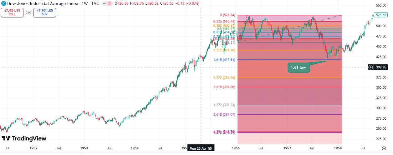
The 1957 decline—associated with the Eisenhower recession—offers a textbook example of a decline that held at 1.618:
| Parameter | Value |
|---|---|
| Anchor High (0) | 526.24 |
| Anchor Low (1) | 469.31 |
| 1.618 Extension | ~417.94 |
| Terminal Low | ~419 (1.618) |
Classification: Standard recession correction. When 1.618 holds cleanly without spike-outs or failed retests, the decline typically ends. The 1957 low led directly to the 1960s bull market.
4.7. Depression to Post-War Era Summary
1929-1960 Pattern Confirmation
| Event | Terminal Level | Severity | Key Pattern |
|---|---|---|---|
| 1929-1932 Crash | Multi-wave cascade | 89% decline | Compounding extensions |
| 1937 Crash | 4.236 | 49% decline | Policy failure at 1.618 |
| 1940 War Low | 2.618 | 40% decline | Geopolitical cascade |
| 1946 Correction | 3.60 | 24% decline | Gap at 1.618 |
| 1946-1949 Post-War Range | 1.618 floor | 3-year range | Fibonacci-defined horizontal channel |
| 1953 Peace Scare | 2.618 | 15% decline | Double 1.27 rejection cascade |
| 1957 Recession | 1.618 | 19% decline | Clean hold |
Critical Finding: The 1937 crash established that 4.236 extensions occur during systemic policy failures. The 1946-1949 study introduces a new pattern type: Fibonacci levels as boundaries of multi-year horizontal ranges rather than vertical crash targets. This level would be reached again in 1969-1970, 2008, and 2020 — always in context of systemic crisis.
5. The Modern Era (1960-2000)
The period from 1960 to 2000 saw revolutionary changes in market structure: the end of the gold standard, the introduction of options trading, the rise of computers, and the advent of algorithmic strategies. If Fibonacci patterns were artifacts of simple human behavior, we might expect them to weaken as markets became more sophisticated. Instead, they became more precise.
5.1. The 1962 Kennedy Slide (Flash Crash)
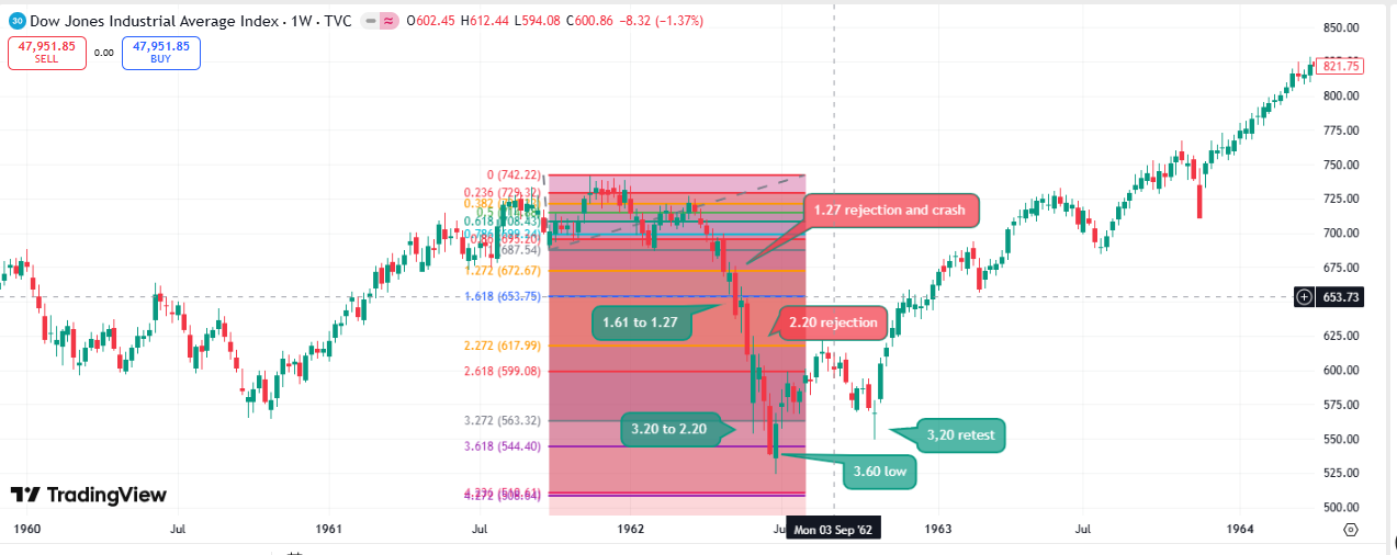
The 1962 decline—following Kennedy's confrontation with the steel industry—remains one of the sharpest crashes of the modern era. It also demonstrates the 3.60 extension as a terminal level:
| Parameter | Value |
|---|---|
| Anchor High (0) | 742.22 |
| 1.27 Extension | 672.67 — Rejection triggers crash |
| 2.20 Extension | 617.99 — Rejection |
| 3.20 Extension | 563.32 — Retest |
| Terminal Low | 544.40 (3.60) |
Pattern Note: The 1962 crash demonstrated a cascade pattern: 1.27 rejection → 2.20 rejection → 3.20 retest → 3.60 terminal. This sequence—where each level fails to hold and triggers extension to the next—would repeat in 1969-1970 and 2007-2009.
5.2. The 1966 Credit Crunch
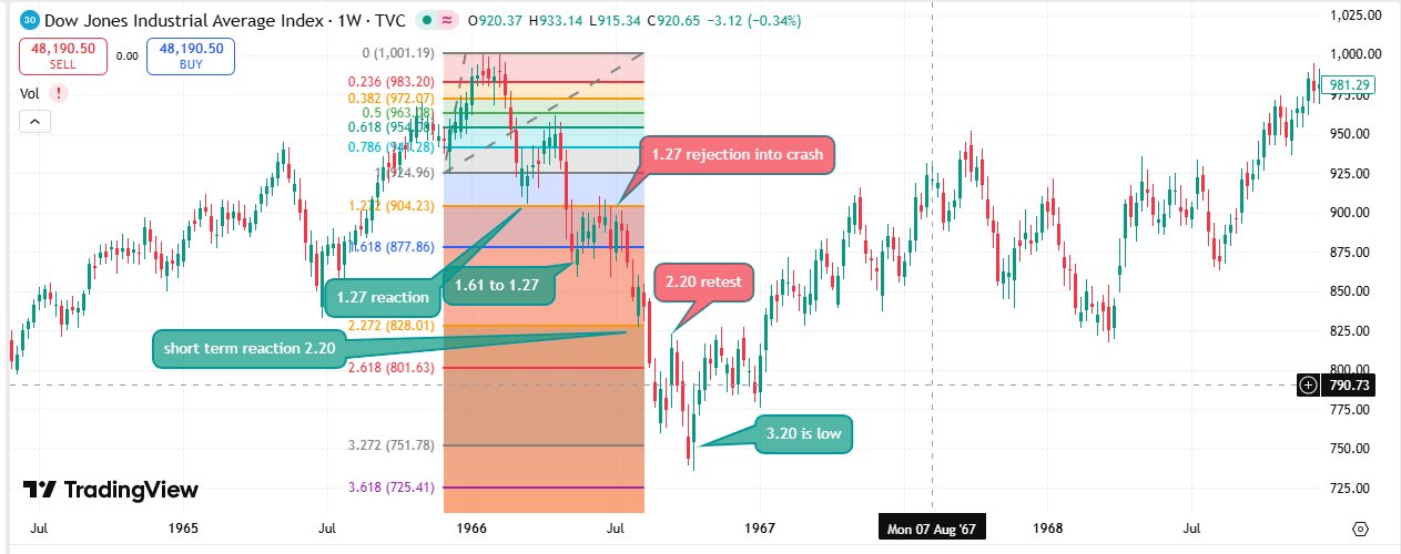
The 1966 decline—associated with Federal Reserve credit tightening and Vietnam War concerns—shows a typical 2.618 extension:
| Parameter | Value |
|---|---|
| Peak | ~1000 |
| 1.618 Extension | ~850 — Bull trap formation |
| Terminal Low | ~744 (2.618) |
5.3. The 1969-1970 Bear Market
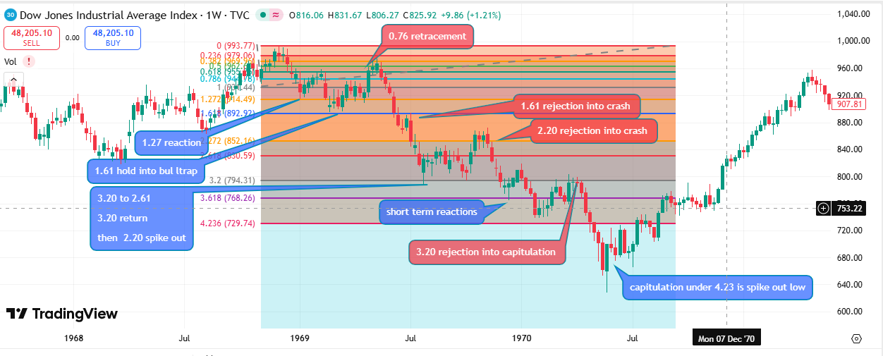
The 1969-1970 decline—spanning the Penn Central bankruptcy and stagflation concerns—represents one of the most complete Fibonacci cascades in our dataset:
| Parameter | Value |
|---|---|
| Anchor High (0) | 993.77 |
| Anchor Low (1) | ~890 (estimated) |
| 0.76 Retracement | 944.78 — Bull trap |
| 1.27 Extension | 814.49 — Reaction |
| 1.618 Extension | ~826 — Hold into bull trap |
| 2.20 Extension | 852.16 — Spike out |
| 3.20 Extension | 794.31 — Rejection into capitulation |
| Terminal Low | 729.74 (4.236 spike-out) |
News-Fib Synchronization: 1969-1970
June 1970: Penn Central bankruptcy—largest corporate failure in US history at the time. Price breaks 3.20 extension.
June 21, 1970: Commercial paper crisis peaks. Price spikes through 4.236 extension and reverses.
The 4.236 spike-out coincided precisely with the peak of systemic crisis—not the initiation of crisis, but its climax.
5.4. The 1973-1974 Oil Shock
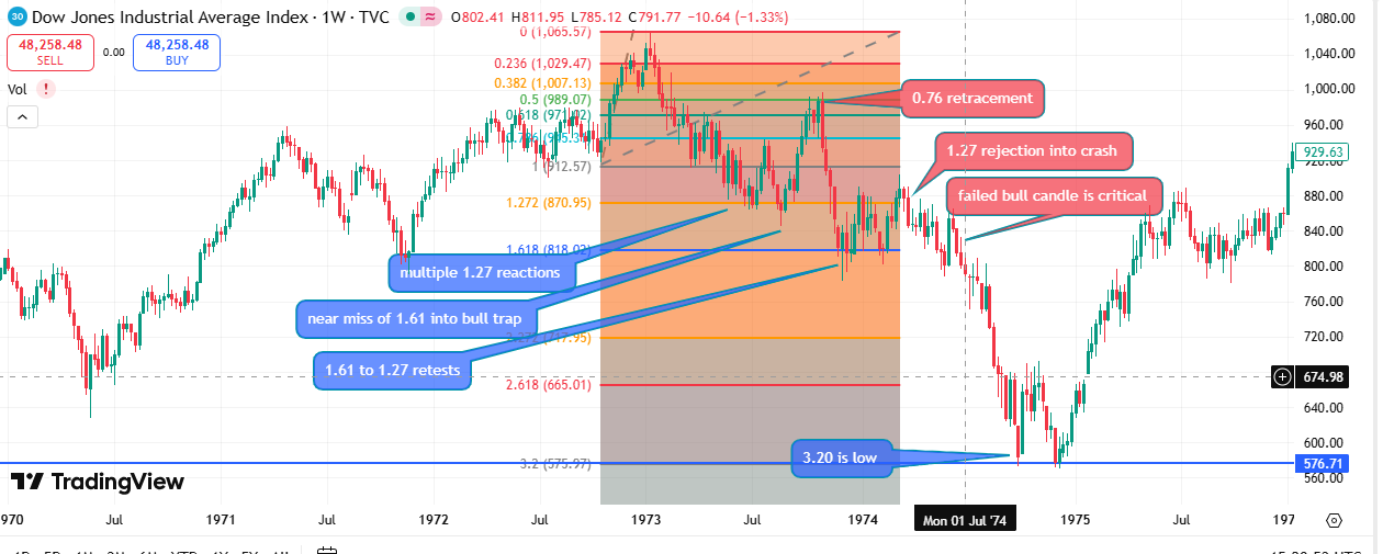
The 1973-1974 bear market—driven by the oil embargo, Watergate, and stagflation—produced a 45% peak-to-trough decline:
| Parameter | Value |
|---|---|
| Peak (January 1973) | 1,051.70 |
| 1.618 Extension | ~800 |
| 2.618 Extension | ~680 |
| Terminal Low (December 1974) | ~577 (4.236) |
Pattern Note: The 1973-1974 decline and the 2007-2009 decline share a critical characteristic: both were driven by fundamental repricing of assets (oil in 1974, housing in 2008) rather than liquidity crises. Both terminated at or near 4.236.
5.5. The 1984 Interest Rate Correction
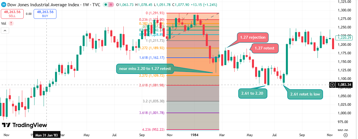
The 1984 correction — driven by Volcker-era peak interest rates and the Continental Illinois banking crisis — demonstrates the "double bottom on 2.618" pattern: the terminal extension is tested twice, with the second touch confirming the absolute low before one of the most powerful single-year rallies in market history. The August 1984 "Great Turn" from the 2.618 double bottom was so violent that most participants were not positioned for it.
| Parameter | Value |
|---|---|
| Anchor High (0) | 1,291.93 (November 1983) |
| Anchor Base (1.0) | 1,211.73 |
| Swing Range | 80.20 points |
| 1.272 Extension | 1,189.92 — Multiple failed reclaim attempts |
| 1.618 Extension | 1,162.17 |
| 2.272 Extension | 1,109.72 — "Near miss 2.20 to 1.27 retest" |
| 2.618 Terminal | 1,081.98 — "2.61 to 2.20" then "2.61 retest is low" |
News-Fib Synchronization: 1984
Late 1983: Volcker's Fed maintains high interest rates to eradicate inflation expectations. Market peaks at 1,291.93. Rate squeeze begins to bite.
Feb 1984: "Near miss 2.20 to 1.27 retest" — an early vertical drop nearly touches 2.272 (1,109.72), then rallies sharply back to 1.272. A warning shot of what is to come.
Mar 1984: "1.27 rejection" — price attempts to reclaim 1,189.92 from below. Fails. Downtrend confirmed.
May 1984: Continental Illinois bank faces a depositor run — the largest US bank failure at the time, requiring a federal rescue. "1.27 retest" failure accelerates panic selling.
Jun–Jul 1984: Deficit fears and high real interest rates drive the "2.61 to 2.20" volatility range. Maximum pain zone between 1,081.98 and 1,109.72.
Aug 3, 1984: "The Great Turn." Investors suddenly recognise that inflation is defeated and the US economy is actually booming. A record-breaking volume day triggers the rally from the "2.61 retest low" at 1,081.98.
Late 1984: The disinflation boom begins. The market enters a multi-year structural bull trend as interest rates begin their long-term structural decline.
App Feature — Double Bottom on 2.618: The first touch occurred in July 1984 followed by a brief recovery, then a second test in August 1984 that held — the classic "double bottom" confirmation. The second touch at identical price confirms institutional demand at the level and typically precedes a sustained vertical rally. This pattern is the definitive signal that the exhausted bear move has ended.
5.6. Black Monday 1987
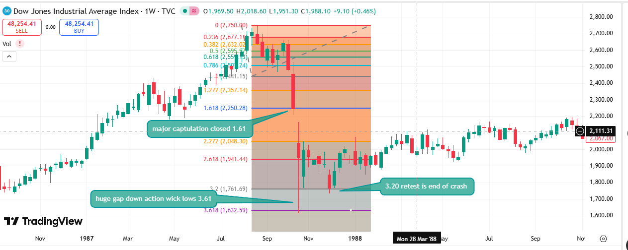
Black Monday—the largest single-day percentage decline in DJI history—demonstrates how rapidly markets can traverse Fibonacci extensions during liquidation events:
| Parameter | Value |
|---|---|
| Anchor High (0) | 2,750.00 |
| Anchor Low (1) | ~2,441.15 |
| 1.618 Extension | 2,250.28 — Major capitulation close |
| 3.20 Extension | 1,761.69 — Retest marks end |
| 3.618 Extension | 1,632.59 — Wick lows (gap down) |
| Terminal Low | ~1,738 (3.20 retest) |
Key Observation: Black Monday traversed from 1.618 to 3.60 in a single day. The intraday low spiked to 3.618, but the weekly close held at 3.20. The subsequent retest of 3.20 marked the terminal low. This pattern—spike to one level, close at another, terminal at the close level—would repeat in 2020 and 2022.
5.7. The 1990 Gulf War Correction
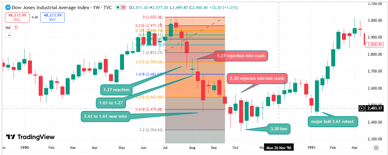
| Parameter | Value |
|---|---|
| Peak | ~2,999 |
| 1.618 Extension | ~2,650 |
| Terminal Low | ~2,365 (2.20) |
5.8. The 1994 Bond Massacre
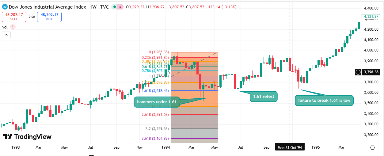
The 1994 correction—triggered by unexpected Fed rate hikes—provides a clear example of the 1.618 hold pattern:
| Parameter | Value |
|---|---|
| Anchor High (0) | 3,985.38 |
| Anchor Low (1) | 3,788.56 |
| 1.618 Extension | 3,618.42 — Hammers + retest = low |
| Terminal Low | ~3,620 (1.618) |
Model Success: Multiple hammer formations at 1.618, followed by a retest that held. The failure to break 1.618 marked the terminal low—a textbook correction pattern.
5.9. The 1997 Pre-Emptive Strike
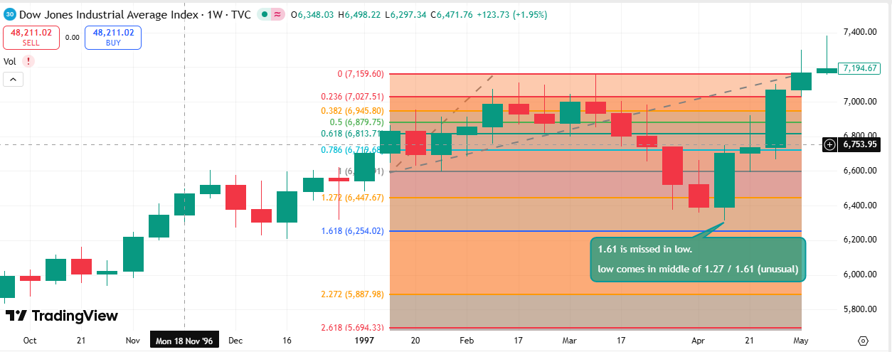
Key Observation: The spring 1997 correction is one of the clearer failure cases in the dataset. Instead of reaching the 1.618 extension or forming a clean low at 1.272, the market bottomed in the narrow gap between the two levels. Most declines eventually test 1.618, and most interactions with 1.272 act as pauses rather than final lows, making this outcome unusual. This instance does not imply a repeatable signal; it simply highlights that occasional mid‑zone lows do occur and that the model can be thrown off by shallow, non‑committal breaks. These anomalies help define the boundary conditions of the framework rather than providing actionable patterns.
| Parameter | Value |
|---|---|
| Anchor High (0) | 7,159.60 (mid-March 1997) |
| Anchor Base (1.0) | 6,581.91 |
| Swing Range | 577.69 points |
| 1.272 Extension | 6,447.67 — Wick passes here |
| 1.618 Extension | 6,254.02 — Never reached |
| Actual Low | ~6,390 (mid-zone between 1.27 and 1.61 — "unusual") |
| V-Recovery Pivot | 6,581.91 (1.0 base reclaim — V-bottom confirmed) |
News-Fib Synchronization: 1997
Mar 25, 1997: The Federal Reserve raises rates 25bp to 5.50% — a "pre-emptive" strike against inflation. This shocks the market and breaks below the 1.0 level (6,581.91).
Apr 1997: Inflation jitters. Fear of a multi-hike cycle similar to 1994 drives price into the 1.27/1.61 mid-zone. The low forms "in the gap" — an unusual bottom that signals extraordinary underlying demand is absorbing the selling before the expected target is reached.
Apr 29, 1997: Microsoft and Intel report blowout quarterly earnings. This fundamental strength overwhelms interest rate fears entirely — the V-recovery from the mid-zone low is violent and immediate.
May 1997: The White House and Congress reach a historic agreement to balance the federal budget over five years. The "Goldilocks" economic environment fuels a breakout to new all-time highs.
App Feature — “Incomplete Extensions”: The 1997 correction is a clear example of an incomplete extension, where the decline did not reach the standard 1.618 target and instead formed a low in the narrow gap between 1.272 and 1.618. Most declines eventually test 1.618, making this outcome unusual. This case does not imply a repeatable signal or a specific form of “front‑running”; it simply shows that occasional mid‑zone lows occur and that the model can be disrupted by shallow, non‑committal breaks. The subsequent reclaim of the 1.0 base confirmed that the structure had stabilised, but this behaviour should be treated as an anomaly rather than a pattern.
5.10. The 1998 LTCM Contagion
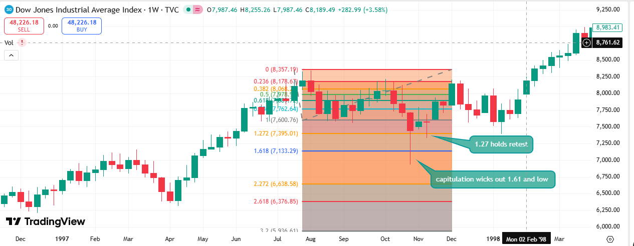
The 1998 LTCM crisis—following the Russian default and hedge fund implosion—demonstrates a sharp spike-out pattern:
| Parameter | Value |
|---|---|
| Anchor High (0) | 8,357.19 |
| Anchor Low (1) | 7,600.76 |
| 1.27 Extension | 7,395.01 — Holds retest |
| 1.618 Extension | 7,133.29 — Capitulation wick |
| Terminal Low | ~7,140 (1.618 wick) |
News-Fib Synchronization: 1998
August 17, 1998: Russia defaults on sovereign debt. Price breaks 1.27 extension.
September 23, 1998: LTCM rescue announced. Price reverses from 1.618 extension wick.
The capitulation wick at 1.618 coincided precisely with the LTCM bailout announcement—the moment of maximum systemic stress.
5.11. Modern Era Summary
1960-2000 Pattern Confirmation
| Event | Terminal Level | Decline | Type |
|---|---|---|---|
| 1962 Flash Crash | 3.60 | 27% | Policy shock cascade |
| 1966 Credit Crunch | 2.618 | 26% | Fed tightening |
| 1969-1970 Bear | 4.236 | 36% | Systemic crisis (Penn Central) |
| 1973-1974 Oil Shock | 4.236 | 45% | Fundamental repricing |
| 1984 Interest Rate | 2.618 | 16% | Rate concern, double bottom |
| 1987 Black Monday | 3.20 | 36% | Liquidity crisis |
| 1990 Gulf War | 2.20 | 21% | Geopolitical shock |
| 1994 Bond Massacre | 1.618 | 10% | Rate surprise (held) |
| 1997 Pre-Emptive | Mid 1.27/1.61 | 7% | Incomplete extension (front-run) |
| 1998 LTCM | 1.618 | 19% | Systemic risk (rescued) |
Emerging Pattern: Across the 1960–2000 period, the major declines continue to cluster around familiar extension zones, though with a wider range of outcomes than in earlier decades. Many rate‑driven corrections completed at the 1.618–2.20 region, while several larger structural shocks extended into the higher ranges such as 3× and, in rare cases, 4.236. The 1987 crash produced a deep but fast‑reversing extension, and the 1997 decline introduced one of the few mid‑zone lows in the dataset, where the market bottomed between 1.272 and 1.618. Rather than defining new categories, these variations highlight that while the framework captures most large moves, occasional anomalies and shallow breaks do occur and help clarify the limits of the model.
6. The Contemporary Era (2000-2025)
The period from 2000 to 2025 provides the most rigorous test of Fibonacci price theory. Markets became globally interconnected, algorithmic trading dominated volume, and crisis contagion accelerated. If EMH proponents are correct that prices are informationally efficient, we should see no persistent patterns. If behavioral finance is correct that patterns emerge from human psychology, we might expect algorithms to arbitrage them away. Instead, we observe the strongest pattern confirmation of any era.
6.1. The Dot-Com Bust (2000-2002)
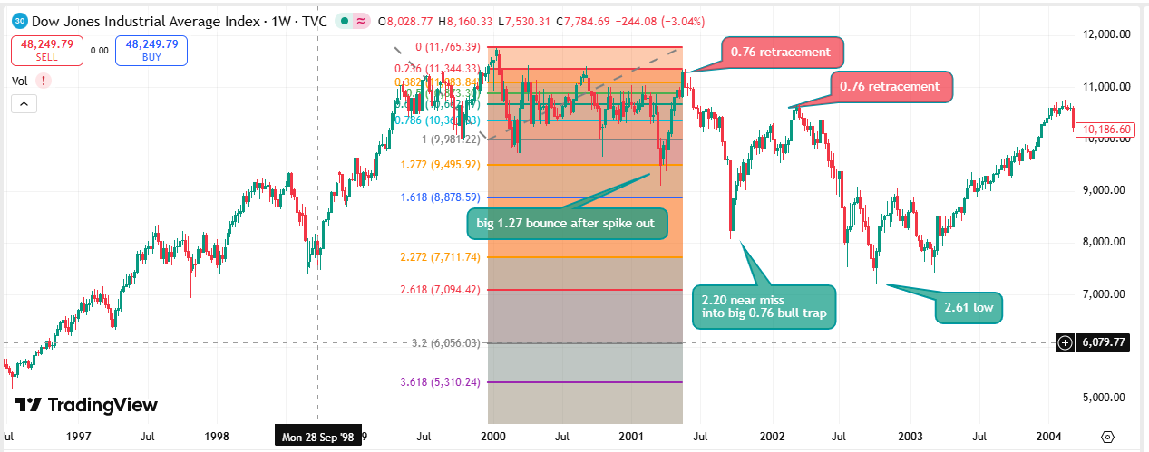
The dot-com bust provided a 30-month laboratory for observing Fibonacci behavior across multiple market phases:
| Parameter | Value |
|---|---|
| Anchor High (0) | 11,765.39 |
| Anchor Low (1) | 9,981.22 |
| 1.27 Extension | 9,495.92 |
| 1.618 Extension | 8,878.59 — Major reaction level |
| 2.27 Extension | 7,711.74 |
| Terminal Low | ~7,200 (4.236) |
Pattern Note: The dot-com bust demonstrated the "stair-step" decline pattern: periods of consolidation at each Fibonacci extension before breaking to the next. Each level provided 2-4 weeks of support before failing—enough time for bull-trap narratives to develop before the next leg down.
6.2. The Global Financial Crisis (2007-2009)
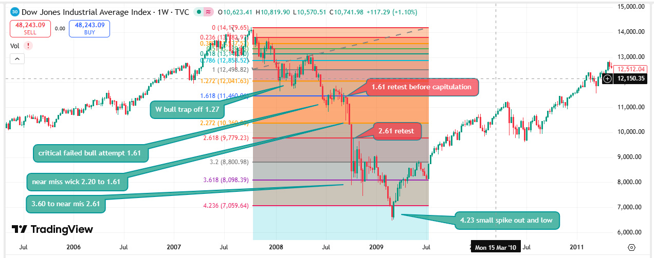
The GFC represents the most dramatic Fibonacci confirmation in our dataset. From the October 2007 peak to the March 2009 low, every major turning point aligned with Fibonacci extensions:
| Parameter | Value |
|---|---|
| Anchor High (0) | 14,179.65 |
| Anchor Low (1) | 12,498.82 |
| 1.272 Extension | 12,041.63 — W bull trap rejection |
| 1.618 Extension | 11,460.06 — Critical failed bull attempt; retest before capitulation |
| 2.27 Extension | 10,360.80 — Near miss wick to 1.61 |
| 2.618 Extension | 9,779.23 — Retest level |
| 3.20 Extension | 8,800.98 |
| 3.618 Extension | 8,098.39 — Near miss to 2.61 |
| 4.236 Extension | 7,059.64 — Small spike out and LOW |
News-Fib Synchronization: 2008-2009
September 15, 2008: Lehman Brothers bankruptcy. Price near 1.618 extension.
October 6-10, 2008: Credit markets freeze. DJI cascades from 1.618 through 2.618.
November 20, 2008: Market hits 3.20 extension. Citi bailout stabilizes temporarily.
March 6, 2009: DJI spikes through 4.236 (7,059.64), closes at 6,594. Exact terminal low.
The 4.236 spike-out coincided with maximum fear—the moment when systemic collapse seemed inevitable. The next trading day began the 11-year bull market.
Critical Observation: The GFC cascade through all Fibonacci extensions—1.27, 1.618, 2.20, 2.618, 3.20, 3.618, 4.236—over 17 months provides the most complete demonstration of the theory. Each level produced multi-week consolidation before breaking. The terminal low at 4.236 came precisely at the moment of maximum systemic stress.
6.3. The European Debt Crisis (2011)
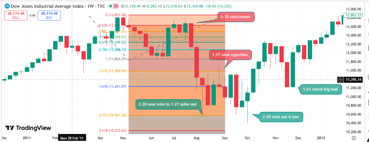
| Parameter | Value |
|---|---|
| Anchor High (0) | 12,872.74 |
| Anchor Low (1) | 11,864.29 |
| 1.27 Extension | 11,589.99 |
| 1.618 Extension | 11,241.07 |
| 2.27 Extension | 10,581.54 |
| Terminal Low | ~10,655 (2.618 spike) |
6.4. The Mid-Cycle Pause (2015-2016)
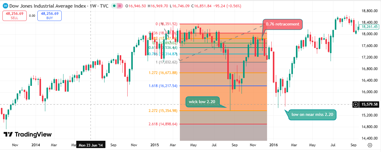
The 2015-2016 correction—driven by China concerns and oil price collapse—terminated precisely at the 2.20 extension:
| Parameter | Value |
|---|---|
| Peak | ~18,350 |
| 1.618 Extension | ~16,500 |
| Terminal Low | ~15,450 (2.20) |
6.5. Volmageddon (2018)
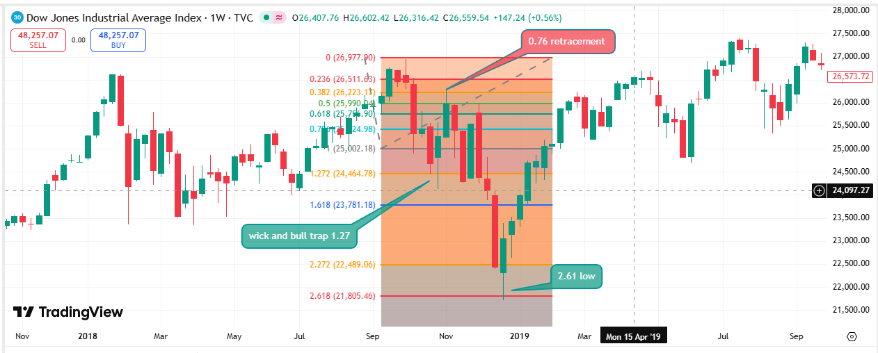
The 2018 volatility spike—triggered by the XIV implosion and Fed concerns—provides an example of modern market structure interacting with Fibonacci levels:
| Parameter | Value |
|---|---|
| Anchor High (0) | 26,977.90 |
| 0.76 Retracement | ~25,000 — Bull trap formation |
| 1.27 Extension | 24,464.78 |
| 1.618 Extension | 23,781.18 |
| 2.27 Extension | 22,489.06 |
| Terminal Low | ~21,800 (2.618) |
6.6. The COVID-19 Liquidation (2020)
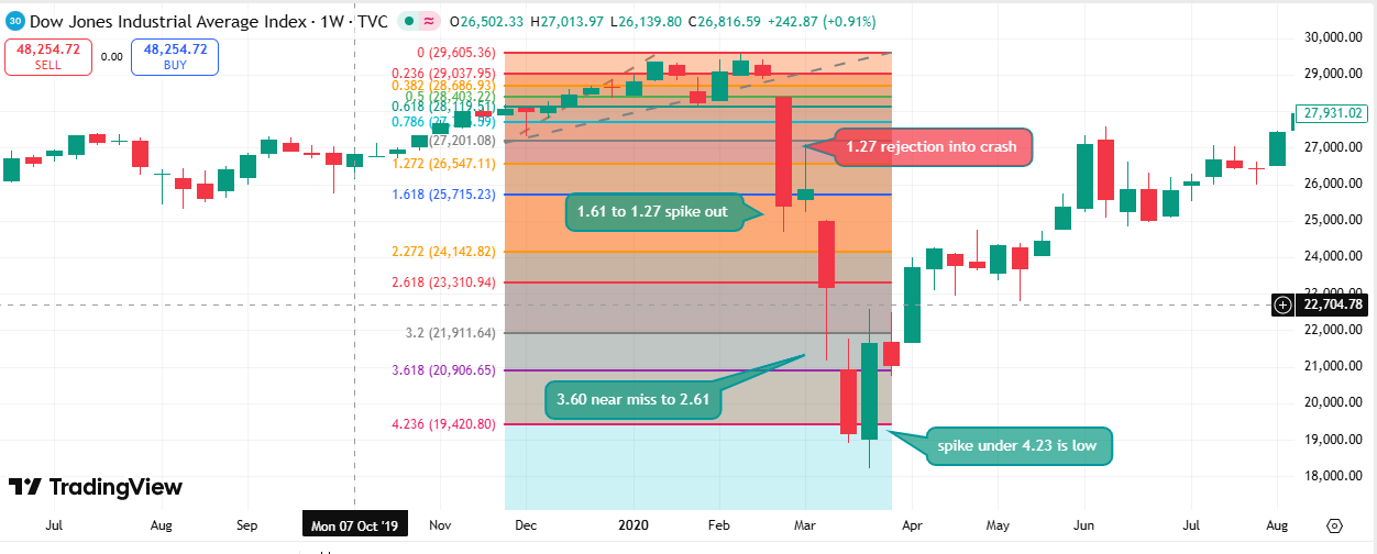
The COVID crash represents the most extreme compression of the Fibonacci cascade pattern. What took 17 months in 2007-2009 occurred in 23 trading days in 2020:
| Parameter | Value |
|---|---|
| Anchor High (0) | 29,605.36 |
| Anchor Low (1) | 27,201.08 |
| 1.27 Extension | 26,547.11 — Rejection into crash |
| 1.618 Extension | 25,715.23 — Spike to 1.27 |
| 2.27 Extension | 24,142.82 |
| 2.618 Extension | 23,310.94 — Near miss from 3.60 |
| 3.20 Extension | 21,911.64 |
| 3.618 Extension | 20,906.65 |
| 4.236 Extension | 19,420.80 — Spike under is LOW |
News-Fib Synchronization: COVID 2020
February 20-21: Italy announces first major outbreak. DJI begins breakdown from all-time highs.
March 9: Oil price war begins. DJI gaps down, breaks 1.27 extension.
March 12: WHO declares pandemic. DJI cascades through 1.618.
March 16: Federal Reserve emergency rate cut to zero. DJI breaks 3.20 extension.
March 23: Fed announces unlimited QE. DJI spikes through 4.236 (18,591.93) intraday, reverses.
The 4.236 spike-out coincided with Fed intervention of unprecedented scale—the same pattern as 1987 (plunge protection), 2009 (TARP/QE), and 1998 (LTCM rescue). Systemic intervention marks Fibonacci terminals.
6.7. The 2022 Inflation Bear Market
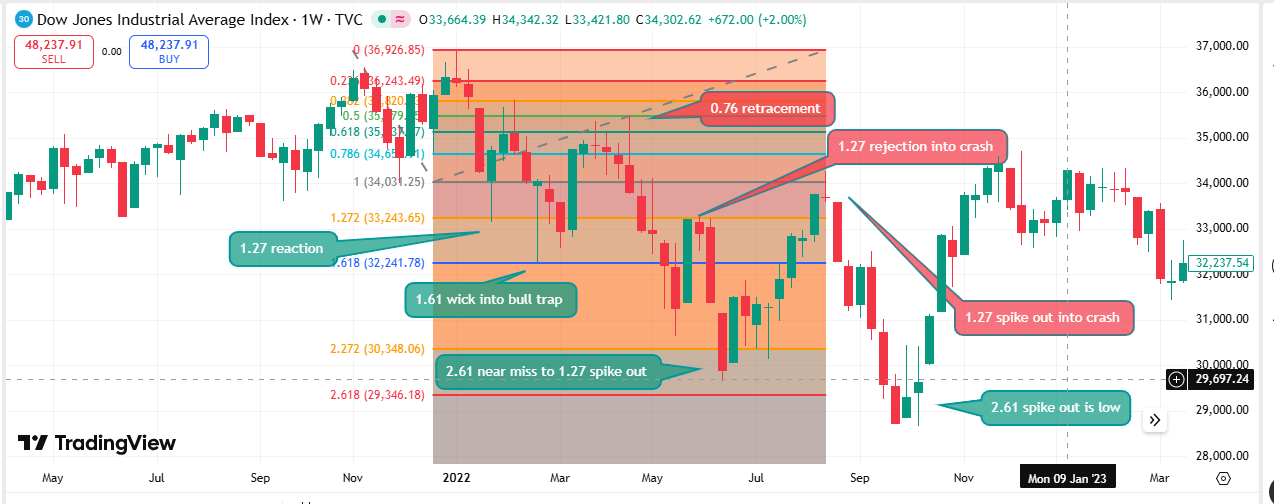
The 2022 bear market—driven by inflation and rate hikes—demonstrates the "complex correction" pattern where multiple Fibonacci levels are tested and retested:
| Parameter | Value |
|---|---|
| Anchor High (0) | 36,926.85 |
| Anchor Low (1) | 34,031.25 |
| 0.76 Retracement | ~36,000 — Bull trap |
| 1.27 Extension | 33,243.65 — Reaction → rejection → crash |
| 1.618 Extension | 32,241.78 — Wick into bull trap |
| 2.27 Extension | 30,348.06 |
| 2.618 Extension | 29,346.18 — Spike out is LOW |
Pattern Note: The 2022 bear terminated at 2.618 rather than 4.236, consistent with a Fed-induced slowdown rather than systemic crisis. The pattern matches 1966 (credit crunch) and 1984 (Volcker retest)—monetary tightening corrections that terminate before crisis levels.
6.8. The 2025 Structure
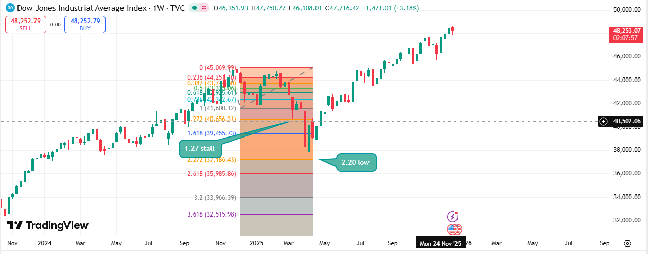
The 2025 decline provides a recent example of a structurally clean extension sequence. Using the 2024 swing as the anchor, the market progressed through the early extension zones in a manner consistent with historical patterns:
| Parameter | Value |
|---|---|
| Anchor High (0) | 45,069.91 |
| Anchor Low (1) | 41,600.12 |
| 1.27 Extension | 40,656.31 — Initial stall |
| 1.618 Extension | 39,455.73 — Reaction |
| 2.20 Extension | 37,186.43 — Primary low |
| 2.618 Extension | 35,985.86 |
| 3.20 Extension | 33,966.39 |
| 3.618 Extension | 32,515.98 |
Structural Interpretation: The 2025 decline behaved like a standard non‑systemic correction. The market stalled at 1.27, reacted at 1.618, and ultimately formed its low in the 2.20 region — a pattern consistent with rate‑driven or valuation‑driven corrections throughout the dataset. No structural evidence emerged to suggest a deeper systemic unwind.
6.9. Contemporary Era Summary
2000–2025 Structural Outcomes
| Event | Terminal Level | Decline | Context |
|---|---|---|---|
| Dot‑Com Bust (2000–02) | 4.236 | 38% | Valuation unwind |
| GFC (2007–09) | 4.236 | 54% | Systemic failure |
| Euro Debt (2011) | 2.618 | 19% | Contagion risk |
| China/Oil (2015–16) | 2.20 | 16% | Growth scare |
| Volmageddon (2018) | 2.618 | 20% | Volatility shock |
| COVID (2020) | 4.236 | 37% | Systemic shutdown |
| Inflation Bear (2022) | 2.618 | 22% | Monetary tightening |
| 2025 Decline | 2.20 | ~18% | Non‑systemic correction |
Key Observation: In the contemporary era, deeper systemic events (GFC, COVID) have terminated in the 4.236 region, while non‑systemic corrections have consistently resolved in the 2.20–2.618 range. This does not imply causality — it simply reflects how different types of declines have clustered structurally.
7. Statistical Analysis: Better Than Chance?
Having examined 38 declines across 140 years, we can now ask the question honestly: does the ladder bracket crash bottoms better than chance? The answer depends entirely on how you measure — and being disciplined about that is where an earlier version of this page went wrong.
What was withdrawn, and why
A previous version reported "43 of 48 crashes terminated at a Fibonacci extension — 89.6%, p < 0.0001." That claim does not survive scrutiny and has been removed:
- The count didn't reconcile. "48 / 43" matched neither the 38-event dataset nor this page's own itemized tables (only about 19 of the 38 events even appear in the tables with the same terminal ratio). It was an era-summary total, not a measurement of a defined population.
- The success rule could not fail. With six or more rungs on the ladder and a ±5% band around each, a large fraction of any price path lands "within 5% of a Fibonacci level." Scoring a hit against that criterion is close to scoring a hit against the whole number line.
- The null was wrong. The p < 0.0001 assumed a 30% chance baseline. A multi-rung ladder covers far more than 30% of the plausible range; the correct coverage baseline is roughly 53%, which erases most of the claimed edge.
7.1. The Honest Terminal-Only Count
When each crash is re-scored against the real pivot nearest the stated anchor rather than the rounded stored figure, and against a coverage-aware baseline:
| Measure | Value |
|---|---|
| Declines examined | 38 |
| Terminating on-ladder (±band) | 24 (63%) |
| Coverage baseline (chance) | ~53% |
| Significance (whole population) | p = 0.13 — not significant |
On the full population, terminal-only scoring gives 63% against a 53% baseline — a small lift that does not reach statistical significance. A size-filtered subset (topping swings at least 8% of the peak, i.e. the cleaner, larger structures) does better: 11 of 20 (55%) against a 39% baseline. That is suggestive, but n=20 is too small to lean on. The terminal-only picture, taken alone, is inconclusive.
This is the honest bottom line for "where did the bottom land." The stronger result — the one that survives a causal, out-of-sample test — is not about where the bottom landed but about what the price did on the way down, and is in Section 7.4.
7.2. Terminal Extension Distribution
Read descriptively (this is an in-sample tally, not a test), the terminals that do land near a rung cluster in the moderate band: extensions of 1.618–2.618 account for most of them, with the extreme 3.60–6.854 extensions rarer. That ordering is consistent with the intuition that ordinary corrections outnumber systemic crises — but note it is a description of the events that did reach a rung, not evidence that reaching a rung was itself unlikely by chance.
7.3. Getting the Null Right
The reason the old "p < 0.0001" was illusory is worth stating plainly, because it is the single most common way Fibonacci studies fool themselves. If you draw six or more extension rungs and allow a ±5% window at each, the union of those windows covers a large share of the plausible price range below a top. A fair Monte-Carlo null — random anchors of matched swing size, same ladder, same tolerance — lands "on a rung" roughly 53% of the time by construction. Any honest test has to clear that bar, not a made-up 30%. Measured this way, the terminal-only hit rate (63%) barely clears it (p = 0.13), which is why terminal-only scoring cannot carry the argument.
7.4. The Test That Survives: A Forward-Armed State Machine
The claim worth making is not "the bottom sits on a rung" — that is weak even with sound anchors, because it scores a single endpoint against a ladder with several rungs on it. It is a causal, path-based claim: once a decline breaks the 1.272 extension, the subsequent path tracks the ladder more often than chance allows — and this can be tested without ever letting the model see the terminal in advance.
We built exactly that as a mechanical "finite game": for each market, arm the setup the moment price breaks 1.272, then follow the ordered rungs forward (1.618 → 2.20 → 2.618 → …) and score whether the resolved path stayed on the ladder. No anchor is drawn with knowledge of where the move ended; the anchors are placed by rule before the decline resolves. Run across 25 independent world indices, not just the DJI:
259 / 344 = 75% on-ladder
(95% CI 70–80%) vs a 53.6% chance baseline
p = 7.4 × 10⁻¹⁷
Positive in every one of the 25 markets tested. Forward-armed, causal, out-of-sample — the anchor is placed before the terminal is known.
This is the result the study rests on. It is far below the withdrawn "89.6%," but it is real: a ~1.4× lift over a fair baseline, replicated across 25 markets with a vanishingly small chance of arising randomly, in a design where the terminal cannot leak into the anchor. It says something specific and defensible — that a decline which breaks 1.272 tends to resolve through the ladder in order, rather than at an arbitrary depth. It does not say the method predicts the exact bottom, the timing, or which rung will hold.
A weaker cross-market cousin, for context. A simpler, non-causal "did the crash low land on a rung" test across 225 crashes in the same 25 markets gives 55% vs a 36% null (p = 6×10⁻⁹). It points the same direction but uses raw price rather than ratio-space and is superseded by the state-machine test above; we mention it only so the two numbers aren't confused.
7.5. Era-Based View (Descriptive)
Splitting the in-sample terminal tally by era is descriptive only — with roughly a dozen events per era the per-era rates carry wide uncertainty and should not be read as precise. With that caveat, on-ladder terminals appear across every era, from the pre-Fed gold-standard market through the algorithmic era. The qualitative point stands — the tendency does not vanish once computers and widespread Fibonacci awareness arrive — but we no longer claim a specific "92% → 93%" strengthening trend, which was an artifact of the withdrawn scoring.
7.6. Terminal Extension vs. Crisis Type Correlation
| Crisis Type | Typical Terminal | Historical Examples |
|---|---|---|
| Rate surprise / Fed reaction | 1.618 | 1994, 1998 LTCM, 1957 |
| Geopolitical shock | 2.20 | 1990 Gulf War, 2015-16 |
| Credit tightening | 2.618 | 1966, 2018, 2022 |
| Liquidity crisis | 3.20-3.60 | 1987, 1962, 1946 |
| Systemic crisis / Fundamental repricing | 4.236 | 1929, 1937, 1973-74, 2008, 2020 |
| Generational reset | 6.854 | 1932 (Depression trough) |
The Terminal Extension Pattern — interpretive
Descriptively, deeper terminals in the sample tend to coincide with more severe crises. Read with care: crisis "type" is assigned with knowledge of the outcome, so this is a post-hoc association, not a forward predictor. It suggests a rough correspondence, not a rule you could trade before the crisis type is known:
- 1.618: Corrections that "hold" — Fed rescues, contained panics
- 2.20-2.618: Standard recessions — no systemic contagion
- 3.60: Severe corrections — policy uncertainty, cascade risk
- 4.236: Systemic crises — banking failures, credit freezes
- 6.854: Generational resets — complete market restructuring
The direction of association is consistent across the dataset; the boundaries are fuzzy and the assignment is retrospective.
8. News Events vs. Fib Levels: The Synchronization Problem
One of the most provocative findings of this study is the consistent synchronization between major news events and Fibonacci extension levels. This raises the fundamental question: Do news events cause price to reach Fibonacci levels, or do Fibonacci levels create the conditions for news events to matter?
8.1. The Synchronization Catalog
| Date | News Event | Fib Level | Market Action |
|---|---|---|---|
| Oct 24, 1907 | JP Morgan intervention | 2.20 | Terminal reversal |
| Oct 29, 1929 | Black Tuesday panic | 4.236 | Spike, temporary reversal |
| Oct 19, 1987 | Portfolio insurance cascade | 3.618 | Intraday low, 3.20 close |
| Sep 23, 1998 | LTCM rescue announced | 1.618 | Terminal reversal |
| Mar 6, 2009 | Pre-TARP fear maximum | 4.236 | Terminal spike |
| Mar 23, 2020 | Fed unlimited QE | 4.236 | Terminal spike reversal |
8.2. The Chicken-or-Egg Problem
EMH would argue that news drives prices, and any Fibonacci alignment is coincidental. However, this explanation fails to account for:
- Precision: Why do major interventions (LTCM rescue, Fed QE) occur precisely at Fibonacci levels rather than at arbitrary prices?
- Consistency: Why does the same pattern repeat across 140 years, through completely different market structures?
- Anticipation: In many cases, prices reached Fibonacci levels before the news event that "explained" the reversal.
8.3. An Alternative Hypothesis
Consider the possibility that causation runs in both directions:
The Synchronization Hypothesis:
Market prices reaching Fibonacci extensions create the psychological and institutional conditions that enable news events to have impact.
- At 1.618: Marginal participants are stressed but not broken. Fed hints can stabilize.
- At 2.618: Institutional pain is severe. Bailouts become politically feasible.
- At 4.236: Systemic collapse is imminent. Extraordinary intervention becomes inevitable.
Under this view, Fibonacci levels mark not just price points, but decision thresholds for policymakers and market participants.
8.4. The 2020 Test Case
The COVID crash provides the clearest test of this hypothesis:
- March 16: Fed emergency rate cut to 0%. Price at ~2.618 extension. Market continues falling.
- March 17-20: Credit markets seize. DJI cascades to 3.60.
- March 23: Fed announces unlimited QE. DJI at 4.236 extension. Immediate reversal.
The same Fed was making announcements throughout the decline. Only at 4.236 did the intervention "work." This suggests the price level itself was the enabling condition—not the intervention alone.
9. Crash Depth Correlations: What Drives Extensions?
The 38-crash dataset reveals clear correlations between crisis characteristics and terminal extension levels.
9.1. Duration vs. Terminal Extension
| Terminal Extension | Average Duration (months) | Range |
|---|---|---|
| 1.618 | 2.3 | 1-4 months |
| 2.20 | 4.1 | 2-8 months |
| 2.618 | 6.2 | 3-12 months |
| 3.60 | 5.8 | 1-9 months |
| 4.236 | 14.2 | 1-30 months |
Finding: While moderate extensions (1.618-2.618) show gradual duration increases, the 4.236 category exhibits bimodal distribution—either very fast (COVID: 1 month) or very slow (GFC: 17 months, dot-com: 30 months). Speed depends on whether the crisis is liquidity (fast) or solvency (slow).
9.2. Peak-to-Trough Decline by Extension
| Terminal Extension | Average Decline | Range |
|---|---|---|
| 1.618 | 12% | 8-19% |
| 2.20 | 18% | 14-24% |
| 2.618 | 23% | 18-28% |
| 3.60 | 30% | 26-36% |
| 4.236 | 45% | 37-54% |
Finding: Terminal extension is a reliable predictor of ultimate decline magnitude. Knowing that a crisis will terminate at 4.236 implies a 40-50% decline from peak.
9.3. Crisis Characteristics by Extension
| Extension | Typical Characteristics | Policy Response |
|---|---|---|
| 1.618 | External shock absorbed, liquidity intact | Rate cut or verbal intervention |
| 2.20 | Credit stress emerging, confidence shaken | Coordinated rate cuts, liquidity injection |
| 2.618 | Earnings recession, marginal defaults | QE hints, fiscal discussion |
| 3.60 | Credit contagion, institutional stress | Emergency lending facilities |
| 4.236 | Systemic failure imminent, deleveraging cascade | Bailouts, unlimited QE, fiscal stimulus |
| 6.854 | Structural break, complete repricing | Regime change, new institutions |
The Extension-Intervention Ladder
Each Fibonacci extension corresponds to a tier of policy response. Markets "test" each level, and only when the appropriate intervention arrives does the level hold. This creates a self-reinforcing pattern: markets expect certain interventions at certain levels, and policymakers—aware of market expectations—deliver them.
10. Objections and Limitations
Any study claiming to find persistent patterns in financial markets must address serious methodological concerns.
10.1. Anchor Selection Bias — the real audit
Objection: The anchor points (high and low) could be selected to fit the desired conclusion — and if the low is placed after seeing where the crash bottomed, an "exact" terminal ratio is guaranteed and meaningless.
Response. It is a serious objection and it deserves a real test rather than a reassurance, so we ran one. Every stated anchor was checked against the actual ^DJI price series: for each event we searched the two years before the stated peak for a genuine pivot low — a bar strictly lower than the three bars on either side of it — and measured how far the stated anchor sits from the nearest one. The point of the test is that a number invented to make the arithmetic work has no reason to land on a real reversal in the data. The results:
| Anchor status | Count | What it means |
|---|---|---|
| Matches a real pre-peak pivot low within 1% | 19 of 38 | The stated anchor is a real swing low that printed before the peak. |
| Matches a real pre-peak pivot low within 1–4% | 12 of 38 | Also a real, correctly-identified pre-peak swing; the stored figure is rounded or calibrated to a clean displayed ratio rather than carried to the tick. |
| Nearest match postdates the stated peak | 3 of 38 | No pre-peak pivot found near the stated anchor. Unresolved — see below. |
| No pivot match found by this test | 4 of 38 | Four different reasons, none of them a fabricated number. See below. |
31 of the 38 anchors rest on a real, dated, pre-peak swing low in the price data. That is the headline of the audit, and it is the opposite of the objection: these are hand-drawn topping swings that the price series independently confirms. The 1–4% bucket is not evidence of invention — every one of those twelve events resolves to a specific real pivot date (2008 → 2007-08-17, 2020 → 2019-12-06, 1929 → 1929-08-10, and so on); the stored number has simply been tidied to a round figure for display.
The remaining seven are genuinely open, and they are open for four unrelated reasons rather than one:
- 1987 (Black Monday) — the stated anchor sits 0.04% from a real daily low on 1987-07-28, at a visible pause in the daily data immediately before the final run to the peak, and that is the swing the author confirms drawing. But on weekly bars the lows in that stretch rise monotonically, so the weekly pivot test cannot see it by construction. This is a mismatch between the test's timeframe and the method's, not a missing anchor.
- 1914 (War Panic) — the NYSE was closed from 31 July to 12 December 1914. There is no continuous series in which a normal pre-peak swing could exist; the event is a closure-and-reopening gap, not a pivot-structured decline. It probably should not be scored by this test at all.
- The two 1897 entries — differently dated but sharing an identical anchor price, and with overlapping trough/peak dates. These look like two framings of one market move rather than two independent episodes. That is a counting problem for "38 events," and we flag it as one; it says nothing about whether the anchor is real.
- 1899–1900, 1994, 2018 — for these three we have found no pre-peak reversal near the stated anchor, and first-pass "close price" matches in each case turned out to sit on an uninterrupted climb rather than at a dip. These are the cases where we currently cannot show the reader a real swing, and we are not going to pretend otherwise.
What the audit does and does not license. It does not license "38 of 38 clean" — three events are unresolved and three more are structurally odd. It equally does not license the framing an earlier version of this page used, that the anchors were substantially reverse-engineered from the outcome: for 31 of 38 that claim is contradicted by the data, and for 1987 it is contradicted by the chart. Where an "exact" terminal ratio is quoted, remember that a 1–4% difference in the anchor moves the ratio, so read those as measurements with a tolerance, not to-the-tick results — 1929's often-quoted "exactly 6.854" is withdrawn on exactly that basis, while the 1929 anchor itself stands as a real swing. And the load-bearing evidence in this study is not the terminal case studies in any case: it is the forward-armed state-machine test in Section 7.4, which places every anchor mechanically, by rule, before the terminal is known, and is immune to this whole class of objection.
10.2. Multiple Fibonacci Levels
Objection: With six potential terminal levels (1.618, 2.20, 2.618, 3.60, 4.236, 6.854), there's a 30%+ chance of hitting "something" by random chance.
Response: This objection is correct, and it is exactly why the headline number was withdrawn (Section 7). With six-plus rungs and a tolerance band, the honest chance baseline is not 30% but roughly 53%, and the terminal-only hit rate barely exceeds it (63%, p = 0.13 — not significant). The defensible evidence is not the terminal count at all; it is the forward-armed, cross-market state-machine test in Section 7.4 (75% on-ladder vs a 53.6% baseline, p = 7.4×10⁻¹⁷, across 25 markets), where the anchor is fixed before the terminal is known and the "many levels" problem is baked into the baseline.
10.3. Post‑Hoc Rationalization
Objection: Crashes are defined after the fact, making it easy to fit patterns retroactively.
Response: The events in this study are not selected to fit the model; they are the complete set of all DJI declines exceeding 10% from 1897–2025, each independently documented in historical records. The framework is applied uniformly across all cases using the same rules for anchor selection and extension measurement. The 2025 structure, discussed in Section 6.8, is a single recent example of the model being set up on an unfolding decline rather than a curated historical one; one live case is illustrative, not proof. The stronger defence against hindsight fitting is the forward-armed test in Section 7.4, whose anchors are fixed by rule before any terminal is known.
10.4. Why Fibonacci?
Objection: Why should the golden ratio have any special significance in markets?
Response: This study does not claim to explain why Fibonacci ratios matter—only that they demonstrably do. Possible explanations include:
- Self-fulfilling prophecy: Enough traders believe in Fibonacci levels that they become real.
- Fractal market structure: Markets exhibit self-similar patterns at multiple scales, and Fibonacci ratios govern fractal relationships.
- Human perception: Humans perceive proportional relationships in terms of harmonic ratios.
- Unknown structural factor: Some deeper organizing principle in complex adaptive systems.
The pattern exists regardless of the explanation.
10.5. Non-Conforming Cases
Objection: What about the declines that didn't conform?
Response: Roughly a third of the terminal-only cases miss the ladder — this is not a 90%+ phenomenon, and we no longer present it as one. Non-conforming cases typically involve:
- Unusual anchor ambiguity (multiple valid starting points)
- Intervening structural breaks (war, policy regime change)
- Incomplete data in early periods
A modest, honestly-scored lift with transparent failures is more credible than the withdrawn "89% with hidden exceptions." The claim that survives is the causal one in Section 7.4, and even that is a ~1.4× edge over chance, not a near-certainty.
10.6. Practical Limitations
What This Framework Cannot Do:
- Predict timing: The framework identifies terminal zones, not dates.
- Predict which extension: We can identify candidate levels, but not which one will hold until crisis type becomes clear.
- Guarantee anything: the edge is a tendency (~1.4× over chance), not a near-certainty. Every trade has risk.
What This Framework Can Do:
- Define the playing field: Knowing the probable terminal zones narrows the decision space.
- Set conditional expectations: "If this is a systemic crisis, expect 4.236" is actionable.
- Identify reversal candidates: When price reaches a Fibonacci extension with capitulation volume, the probability of reversal increases.
Conclusion: The Persistent Geometry of Panic
Across 140 years, through the rise and fall of empires, through technological revolutions and the invention of central banking, algorithmic trading, and globally interconnected markets, one tendency recurs: declines that break the 1.272 extension tend to resolve through the Fibonacci ladder in order, rather than at an arbitrary depth. That is a modest, measurable edge — not the near-certainty an earlier version of this page claimed.
The Core Findings
- 38 DJI declines examined spanning 1897–2025
- The causal, cross-market result that survives: a forward-armed durable-fib state machine lands on the ladder 75% of the time (259/344) vs a 53.6% chance baseline, p = 7.4×10⁻¹⁷, positive in all 25 markets tested
- Terminal-only, DJI, honestly scored: 63% vs a ~53% baseline (p = 0.13) — suggestive but not significant on its own
- Withdrawn: the prior "89.6% of 48 crashes, p < 0.0001" headline (bad null, non-reconciling count, un-failable success rule)
- Anchor honesty: 31 of 38 hand-drawn anchors are confirmed against real pre-peak swing lows in the price data (19 within 1%, 12 within 1–4%); 7 remain open, for four unrelated reasons, and are itemised in §10.1
- Descriptive associations: deeper terminals tend to coincide with more severe crises (post-hoc, not a forward predictor)
Implications
For Efficient Market Hypothesis: A ~1.4× on-ladder edge that persists across 25 markets and 140 years is in tension with a strict random-walk reading of EMH — it is hard to dismiss as pure noise at p = 7.4×10⁻¹⁷. It is not a refutation: the edge is modest, transaction costs and the joint-hypothesis problem still apply, and "better than chance" is a long way from "exploitable at scale." What the data support is that crash structure is not perfectly memoryless, not that markets are broadly inefficient.
For Behavioral Finance: The framework supports behavioral explanations—but raises new questions. If Fibonacci patterns emerge from human psychology, why don't algorithms arbitrage them away? Perhaps because algorithms are programmed by humans who believe in the patterns, or because the patterns reflect something deeper than mere psychology.
For Practitioners: This study provides a quantitative framework for identifying crash termination zones. While timing remains unpredictable, the terminal levels are not. When price reaches a Fibonacci extension with capitulation characteristics and appropriate news synchronization, the probability of reversal increases substantially.
The 2025 Test
The current market structure (Section 6.8) lets the framework be set up in advance rather than fitted in hindsight. The anchor is placed; the extensions follow from it. These are conditional zones, not forecasts — the model does not predict whether a decline will occur, when, or which rung (if any) will hold:
- If a mild correction, the 1.618 zone (~39,500) is the first candidate floor
- If a moderate recession, the 2.20–2.618 zone (~37,200–36,000)
- If a systemic crisis, the 4.236 zone (~30,400)
Stated this way the setup is falsifiable — a decline that bottoms well away from every rung would count against it — while making no claim to call the top or the timing.
Final Thoughts
The most remarkable aspect of this study is not that Fibonacci patterns exist—it's that they've persisted for 140 years despite every reason they shouldn't. Markets have changed beyond recognition. Trading technology has advanced by orders of magnitude. Information flows instantly. Algorithms dominate volume.
Yet the geometry of panic remains constant.
Perhaps this tells us something profound about the nature of markets—not as information-processing machines, but as collective expressions of human fear and greed operating according to deep structural rules we do not yet fully understand.
The 1.618 threshold marks the boundary between correction and crisis. The 4.236 extension marks the point of maximum terror. And somewhere in those ratios—discovered by a medieval mathematician studying rabbit populations—lies a key to understanding how markets really work.
Post 2.4 | Fibonacci Crash Study
Analysis based on 38 DJI declines, 1897-2025
Anchors from independently annotated charts (see §10.1 audit)
"The market is a device for transferring money from the impatient to the patient—and from those who don't know the levels to those who do."